Problems

This section covers Problem classes in more detail.

Class Summary

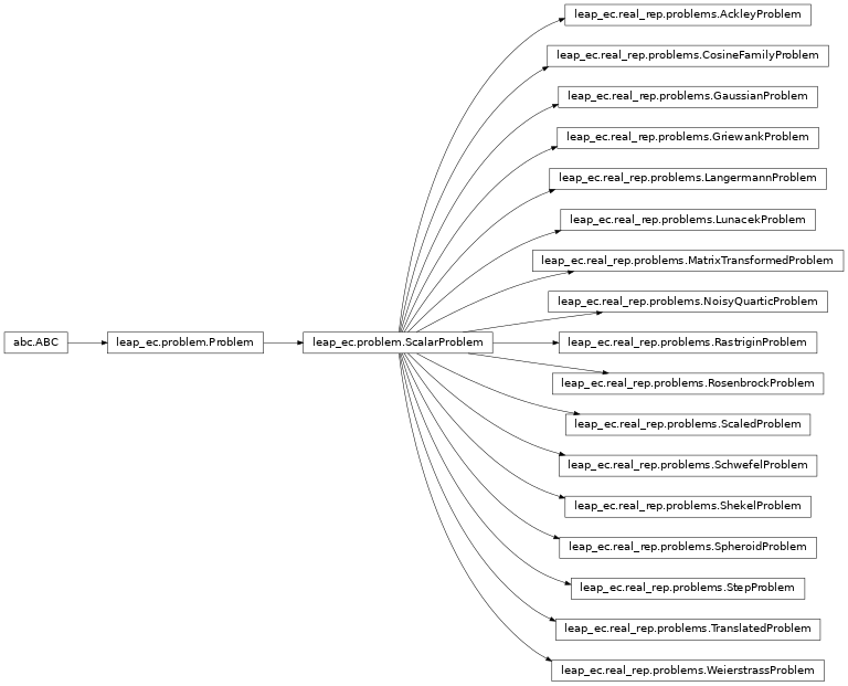
Figure 1: The `Problem` abstract-base class This class diagram shows the detail for Problem, which is an abstract base class (ABC). It has three abstract methods that must be over-ridden by subclasses. evaluate() takes a phenome from an individual and compute a fitness from that. worse_than() and equivalent() compare fitnesses from two different individuals and, as the name suggests, respectively returns the worst of the two or the equivalent within the Problem context.

As shown in Fig. 1, the Problem`abstract-base class has three abstract methods. `evaluate() takes a phenome that was decode()d from an Individual’s genome, and returns a value denoting the quality, or fitness, of that individual. Problems are also used to compare the fitnesses between Individuals. worse_than() returns true if the first individual is less fit than the second. Similarly, equivalent() is used to determine if two given fitnesses are effectively the same.

Class API

Defines the abstract-base classes Problem, ScalarProblem, and FunctionProblem.

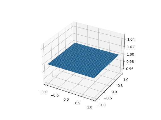
class leap_ec.problem.ConstantProblem(maximize=False, c=1.0)

A flat landscape, where all phenotypes have the same fitness.

This is sometimes useful for sanity checks or as a control in certain kinds of research.

\[f(\vec{x}) = c\]

Parameters

c (float) – the fitness value to return for any input.

from leap_ec.problem import ConstantProblem
from leap_ec.real_rep.problems import plot_2d_problem
bounds = ConstantProblem.bounds
plot_2d_problem(ConstantProblem(), xlim=bounds, ylim=bounds, granularity=0.025)

(Source code, png, hires.png, pdf)

bounds = (-1.0, 1.0)

evaluate(phenome, *args, **kwargs)

Return a contant value for any input phenome:

>>> phenome = [0.5, 0.8, 1.5]
>>> ConstantProblem().evaluate(phenome)
1.0

>>> ConstantProblem(c=500.0).evaluate('foo bar')
500.0

Parameters

phenome – real-valued vector to be evaluated

Returns

1.0, or the constant defined in the constructor

class leap_ec.problem.FunctionProblem(fitness_function, maximize)

evaluate(phenome, *args, **kwargs)

Decode and evaluate the given individual based on its genome.

Practitioners must over-ride this member function.

Note that by default the individual comparison operators assume a maximization problem; if this is a minimization problem, then just negate the value when returning the fitness.

Parameters

phenome –

Returns

fitness

class leap_ec.problem.Problem

Abstract Base Class used to define problem definitions.

A Problem is in charge of two major parts of an EA’s behavior:

1. Fitness evaluation (the evaluate() method)

2. Fitness comparision (the worse_than() and equivalent() methods)

abstract equivalent(first_fitness, second_fitness)

abstract evaluate(phenome, *args, **kwargs)

Decode and evaluate the given individual based on its genome.

Practitioners must over-ride this member function.

Note that by default the individual comparison operators assume a maximization problem; if this is a minimization problem, then just negate the value when returning the fitness.

Parameters

phenome –

Returns

fitness

abstract worse_than(first_fitness, second_fitness)

class leap_ec.problem.ScalarProblem(maximize)

equivalent(first_fitness, second_fitness)

Used in Individual.__eq__().

By default returns first.fitness== second.fitness. Please over-ride if this does not hold for your problem.

Returns

true if the first individual is equal to the second

worse_than(first_fitness, second_fitness)

Used in Individual.__lt__().

By default returns first_fitness < second_fitness if a maximization problem, else first_fitness > second_fitness if a minimization problem. Please over-ride if this does not hold for your problem.

Returns

true if the first individual is less fit than the second

Binary Problems API

A set of standard EA problems that rely on a binary-representation

class leap_ec.binary_rep.problems.ImageProblem(path, maximize=True, size=100, 100)

A variation on max_ones that uses an external image file to define a binary target pattern.

evaluate(phenome)

Decode and evaluate the given individual based on its genome.

Practitioners must over-ride this member function.

Note that by default the individual comparison operators assume a maximization problem; if this is a minimization problem, then just negate the value when returning the fitness.

Parameters

phenome –

Returns

fitness

class leap_ec.binary_rep.problems.MaxOnes(maximize=True)

Implementation of MAX ONES problem where the individuals are represented by a bit vector

We don’t need an encoder since the raw genome is already in the phenotypic space.

evaluate(phenome)

>>> from leap_ec.individual import Individual
>>> from leap_ec.decoder import IdentityDecoder
>>> p = MaxOnes()
>>> ind = Individual([0, 0, 1, 1, 0, 1, 0, 1, 1],
...                   decoder=IdentityDecoder(),
...                   problem=p)
>>> p.evaluate(ind.decode())
5

Real-value Problems API

This module contains a variety of classic real-valued optimization problems that frequently occur in research benchmarks.

It also contains helpers for translating, rotating, and visualizing them.

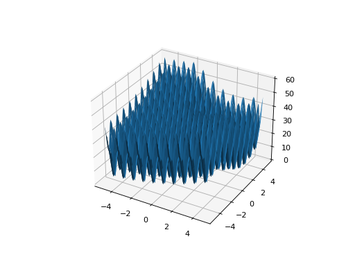
class leap_ec.real_rep.problems.AckleyProblem(a=20, b=0.2, c=6.283185307179586, maximize=False)

\[f(\mathbf{x}) = -a \exp \left( -b \sqrt \frac{1}{d} \sum_{i=1}^d x_i^2 \right) - \exp \left( \frac{1}{d} \sum_{i=1}^d \cos(cx_i) \right) + a + \exp(1)\]

Parameters

• a (float) – depth parameter for the bowl-shaped macrostructure

• b (float) – exponential scale parameter for the bowl

• c (float) – wavenumber (frequency) of the cosine pattern of local optima

• maximize (bool) – the function is maximized if True, else minimized.

from leap_ec.real_rep.problems import AckleyProblem, plot_2d_problem
import math
problem = AckleyProblem(a=20, b=0.2, c=2*math.pi)
bounds = AckleyProblem.bounds  # Contains traditional bounds
plot_2d_problem(problem, xlim=bounds, ylim=bounds, granularity=0.25)

(Source code, png, hires.png, pdf)

bounds = [-32.768, 32.768]

evaluate(phenome)

Computes the function value from a real-valued phenome.

Parameters

phenome – real-valued vector to be evaluated

Returns

its fitness.

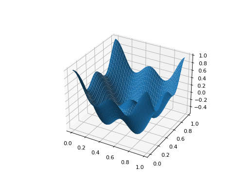
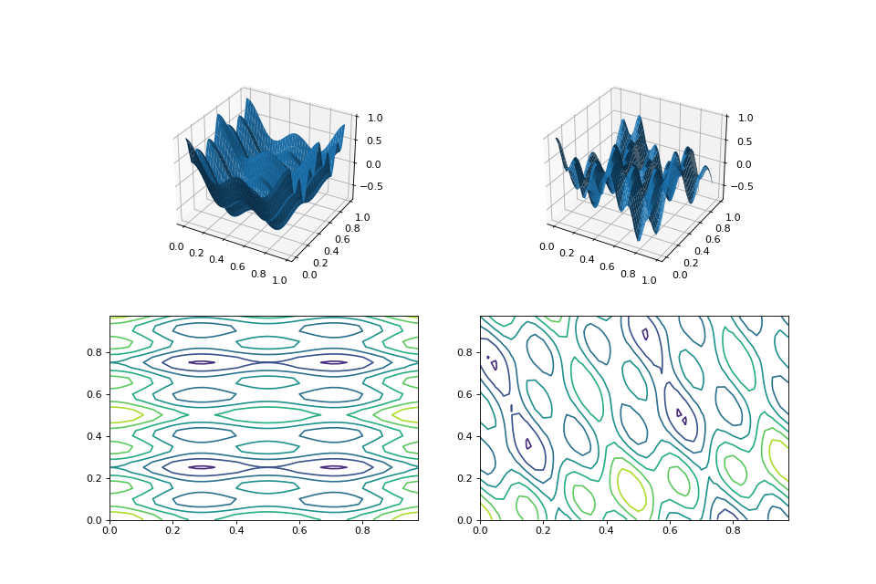
class leap_ec.real_rep.problems.CosineFamilyProblem(alpha, global_optima_counts, local_optima_counts, maximize=False)

A configurable multi-modal function based on combinations of cosines, taken from the problem generators proposed in

Jani2008

“A Generator for Multimodal Test Functions with Multiple Global Optima,” Jani Rönkkönen et al., Asia-Pacific Conference on Simulated Evolution and Learning. Springer, Berlin, Heidelberg, 2008.

[Jani2008]

\[f_{\cos}(\mathbf{x}) = \frac{\sum_{i=1}^n -\cos((G_i - 1)2 \pi x_i) - \alpha \cdot \cos((G_i - 1)2 \pi L-i x_y)}{2n}\]

where \(G_i\) and \(L_i\) are parameters that indicate the number of global and local optima, respectively, in the ith dimension.

Parameters

• alpha (float) – parameter that controls the depth of the local optima.

• global_optima_counts ([int]) – list of integers indicating the number of global optima for each dimension.

• local_optima_counts ([int]) – list of integers indicated the number of local optima for each dimension.

• maximize – the function is maximized if True, else minimized.

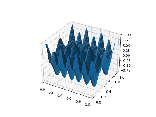
from leap_ec.real_rep.problems import CosineFamilyProblem, plot_2d_problem
problem = CosineFamilyProblem(alpha=1.0, global_optima_counts=[2, 2], local_optima_counts=[2, 2])
bounds = CosineFamilyProblem.bounds  # Contains traditional bounds
plot_2d_problem(problem, xlim=bounds, ylim=bounds, granularity=0.025)

(Source code, png, hires.png, pdf)

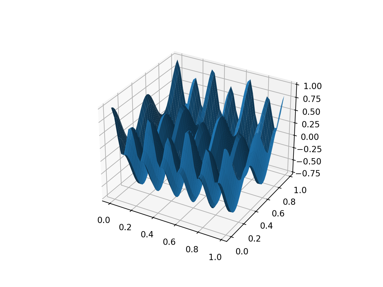
The number of optima can be varied independently by each dimension:

from leap_ec.real_rep.problems import CosineFamilyProblem, plot_2d_problem
problem = CosineFamilyProblem(alpha=3.0, global_optima_counts=[4, 2], local_optima_counts=[2, 2])
bounds = CosineFamilyProblem.bounds  # Contains traditional bounds
plot_2d_problem(problem, xlim=bounds, ylim=bounds, granularity=0.025)

(Source code, png, hires.png, pdf)

bounds = (0, 1)

evaluate(phenome)

Computes the function value from a real-valued phenome.

Parameters

phenome – real-valued vector to be evaluated

Returns

its fitness.

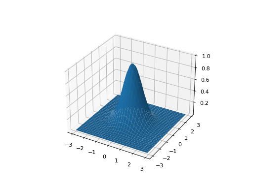
class leap_ec.real_rep.problems.GaussianProblem(width=1, height=1, maximize=True)

A multidimensional, isotropic Gaussian function, defined by

\[A\exp\left( - \sum_i^n \left(\frac{x_i}{w}\right)^2 \right)\]

Parameters

• width (float) – the width parameter \(w\)

• height (float) – the height parameter \(A\)

from leap_ec.real_rep.problems import GaussianProblem, plot_2d_problem
bounds = GaussianProblem.bounds  # Some typical bounds
problem = GaussianProblem(width=1, height=1)
plot_2d_problem(problem, xlim=bounds, ylim=bounds, granularity=0.1)

(Source code, png, hires.png, pdf)

bounds = (-3, 3)

evaluate(phenome)

Decode and evaluate the given individual based on its genome.

Practitioners must over-ride this member function.

Note that by default the individual comparison operators assume a maximization problem; if this is a minimization problem, then just negate the value when returning the fitness.

Parameters

phenome –

Returns

fitness

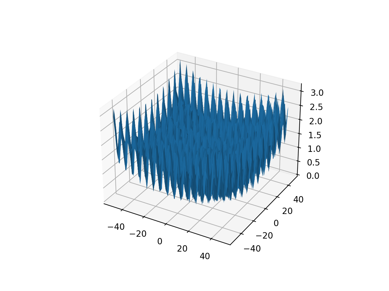
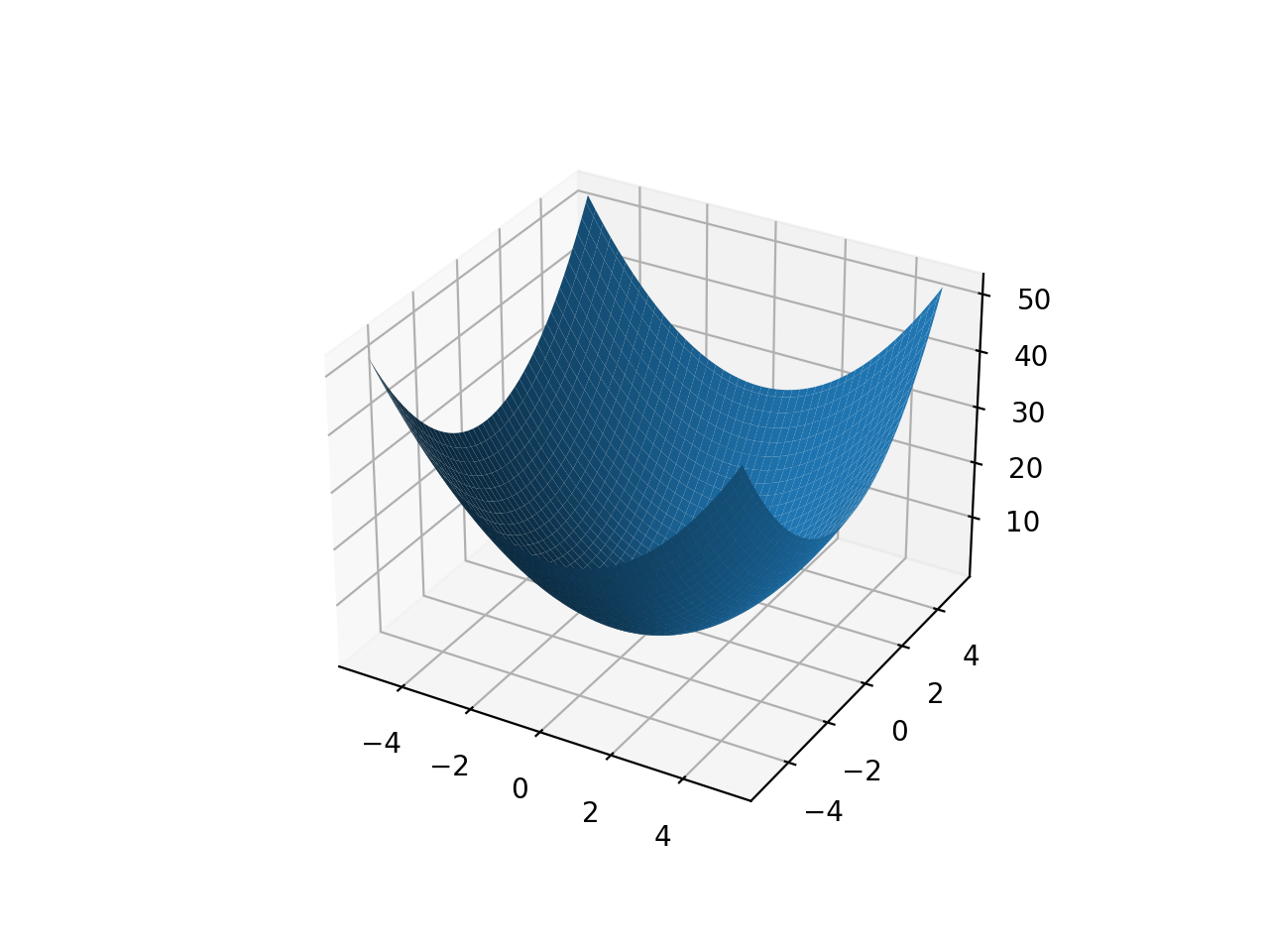
class leap_ec.real_rep.problems.GriewankProblem(maximize=False)

The classic Griewank problem. Like the RastriginProblem function, the Griewank has a quadratic global structure with many local optima that are distributed in a regular pattern.

\[f(\mathbf{x}) = \sum_{i=1}^d \frac{x_i^2}{4000} - \prod_{i=1}^d \cos\left(\frac{x_i}{\sqrt{i}}\right) + 1\]

Parameters

maximize (bool) – the function is maximized if True, else minimized.

from leap_ec.real_rep.problems import GriewankProblem, plot_2d_problem
bounds = GriewankProblem.bounds  # Contains traditional bounds
plot_2d_problem(GriewankProblem(), xlim=bounds, ylim=bounds, granularity=10)

(Source code, png, hires.png, pdf)

from leap_ec.real_rep.problems import GriewankProblem, plot_2d_problem
bounds = [-50, 50]
plot_2d_problem(GriewankProblem(), xlim=bounds, ylim=bounds, granularity=1)

(Source code, png, hires.png, pdf)

bounds = [-600, 600]

evaluate(phenome)

Computes the function value from a real-valued phenome.

Parameters

phenome – real-valued vector to be evaluated

Returns

its fitness.

class leap_ec.real_rep.problems.LangermannProblem(m=5, c=1, 2, 5, 2, 3, a=3, 5, 5, 2, 2, 1, 1, 4, 7, 9, maximize=False)

A popular multi-modal test function built by summing together \(m\) terms.

\[f(\mathbf{x}) = -\sum_{i=1}^m c_i \exp\left( -\frac{1}{\pi} \sum_{j=1}^d(x_j - A_{ij})^2\right) \cos\left(\pi\sum_{j=1}^d(x_j - A_{ij})^2\right)\]

Langermann’s function is parameterized by a vector \(c_i\) of length \(m\) and a matrix \(A_{ij}\) of dimension \(m \times d\). This class uses the traditional parameterization as the default, with \(m=5\) and

\[\begin{split}c = (1, 2, 5, 2, 3) \\ A = \left[ \begin{array}{ll} 3 & 5\\ 5 & 2\\ 2 & 1\\ 1 & 4\\ 7 & 9 \end{array} \right].\end{split}\]

Parameters

• m (int) – total number of terms in the function’s sum

• c ([float]) – amplitude coefficients for each term

• a ([[float]]) – offsets points for each term

• maximize (bool) – the function is maximized if True, else minimized.

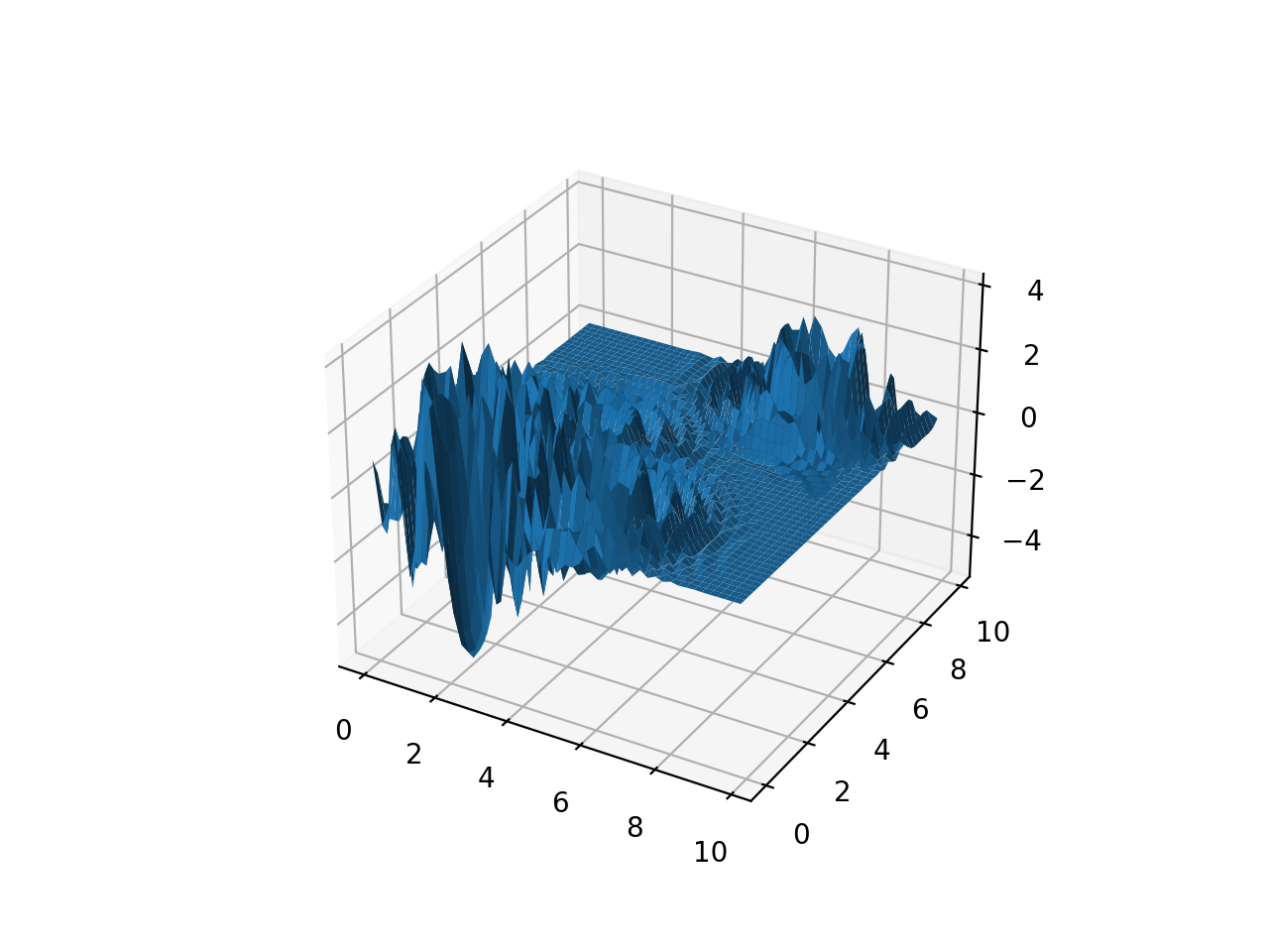
from leap_ec.real_rep.problems import LangermannProblem, plot_2d_problem
bounds = LangermannProblem.bounds  # Contains traditional bounds
plot_2d_problem(LangermannProblem(), xlim=bounds, ylim=bounds, granularity=0.2)

(Source code, png, hires.png, pdf)

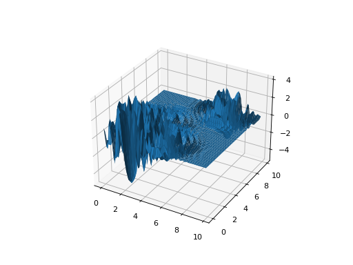
bounds = [0, 10]

default_a = ((3, 5), (5, 2), (2, 1), (1, 4), (7, 9))

evaluate(phenome)

Computes the function value from a real-valued phenome.

Parameters

phenome – real-valued vector to be evaluated

Returns

its fitness.

class leap_ec.real_rep.problems.LunacekProblem(N, d=1.0, mu_1=2.5, mu_2=None, s=None, maximize=False)

Lunacek’s function is also know as the “double Rastrigin” or “bi-Rastrigin” problem, because it overlays a RastriginProblem-style cosine function across a pair of spheroid functions.

This function was designed to model the double-funnel macrostructure that occurs in some difficult cases of the Lennard-Jones function (a famous function from molecular dynamics).

\[f(\mathbf{x}) = \min \left( \left\{ \sum_{i=1}^N(x_i - \mu_1)^2 \right\}, \left\{ d \cdot N + s \cdot \sum_{i=1}^N(x_i - \mu_2)^2\right\} \right) + 10\sum_{i=1}^N(1 - \cos(2\pi(x_i-\mu_i))),\]

where \(N\) is the dimensionality of the solution vector, and the second sphere center parameter \(\mu_2\) is typically given by

\[\mu_2 = -\sqrt{\frac{\mu_1^2 - d}{s}}\]

and \(s\) is by default a function on \(N\):

\[s = 1 - \frac{1}{2\sqrt{N + 20} - 8.2}\]

These respective defaults are used for \(\mu_2\) and \(s\) whenever mu_2 and s are set to None.

Because of these complicated defaults, this class requires that you explicitly set the dimensionality of \(N\) of the expected input solutions. A warning will be thrown if an input solution is encountered that doesn’t match the expected dimensionality.

Parameters

• N (int) – dimensionality of the anticipated input solutions

• d (float) – base fitness value of the second spheroid

• mu_1 (float) – offset of the first spheroid

• mu_2 (float) – offset of the second spheroid (if None, this will be calculated automatically)

• s (float) – scale parameter for the second spheroid (if None, this will be calculated automatically)

• maximize (bool) – the function is maximized if True, else minimized.

from leap_ec.real_rep.problems import LunacekProblem, plot_2d_problem
bounds = LunacekProblem.bounds  # Contains traditional bounds
plot_2d_problem(LunacekProblem(N=2), xlim=bounds, ylim=bounds, granularity=0.1)

(Source code, png, hires.png, pdf)

bounds = (-5, 5)

evaluate(phenome)

Computes the function value from a real-valued phenome.

Parameters

phenome – real-valued vector to be evaluated

Returns

its fitness.

class leap_ec.real_rep.problems.MatrixTransformedProblem(problem, matrix, maximize=None)

Apply a linear transformation to a fitness function.

Parameters

matrix – an nxn matrix, where n is the genome length.

Returns

a function that first applies -matrix to the input, then applies fun to the transformed input.

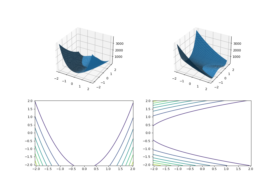
For example, here we manually construct a 2x2 rotation matrix and apply it to the leap.RosenbrockProblem function:

from matplotlib import pyplot as plt
from leap_ec.real_rep.problems import RosenbrockProblem, MatrixTransformedProblem, plot_2d_problem

original_problem = RosenbrockProblem()
theta = np.pi/2
matrix = [[np.cos(theta), -np.sin(theta)],                 [np.sin(theta), np.cos(theta)]]

transformed_problem = MatrixTransformedProblem(original_problem, matrix)

fig = plt.figure(figsize=(12, 8))

plt.subplot(221, projection='3d')
bounds = RosenbrockProblem.bounds  # Contains traditional bounds
plot_2d_problem(original_problem, xlim=bounds, ylim=bounds, ax=plt.gca(), granularity=0.025)

plt.subplot(222, projection='3d')
plot_2d_problem(transformed_problem, xlim=bounds, ylim=bounds, ax=plt.gca(), granularity=0.025)

plt.subplot(223)
plot_2d_problem(original_problem, kind='contour', xlim=bounds, ylim=bounds, ax=plt.gca(), granularity=0.025)

plt.subplot(224)
plot_2d_problem(transformed_problem, kind='contour', xlim=bounds, ylim=bounds, ax=plt.gca(), granularity=0.025)

(Source code, png, hires.png, pdf)

evaluate(phenome)

Evaluated the fitness of a point on the transformed fitness landscape.

For example, consider a sphere function whose global optimum is situated at (0, 1):

>>> s = TranslatedProblem(SpheroidProblem(), offset=[0, 1])
>>> round(s.evaluate([0, 1]), 5)
0

Now let’s take a rotation matrix that transforms the space by pi/2 radians:

>>> import numpy as np
>>> theta = np.pi/2
>>> matrix = [[np.cos(theta), -np.sin(theta)],                      [np.sin(theta), np.cos(theta)]]
>>> r = MatrixTransformedProblem(s, matrix)

The rotation has moved the new global optimum to (1, 0)

>>> round(r.evaluate([1, 0]), 5)
0.0

The point (0, 1) lies at a distance of sqrt(2) from the new optimum, and has a fitness of 2:

>>> round(r.evaluate([0, 1]), 5)
2.0

classmethod random_orthonormal(problem, dimensions, maximize=None)

Create a MatrixTransformedProblem that performs a random rotation and/or inversion of the function.

We accomplish this by generating a random orthonormal basis for R^n and plugging the resulting matrix into MatrixTransformedProblem.

The classic algorithm we use here is based on the Gramm-Schmidt process: we first generate a set of random vectors, and then convert them into an orthonormal basis. This approach is described in Hansen and Ostermeier’s original CMA-ES paper:

“Completely derandomized self-adaptation in evolution strategies.” Evolutionary Computation 9.2 (2001): 159-195.

Parameters

• problem – the original ScalarProblem to apply the transform to.

• dimensions (int) – the number of elements each vector should have.

• maximize (bool) – whether to maximize or minimize the resulting fitness function. Defaults to whatever setting the underlying problem uses.

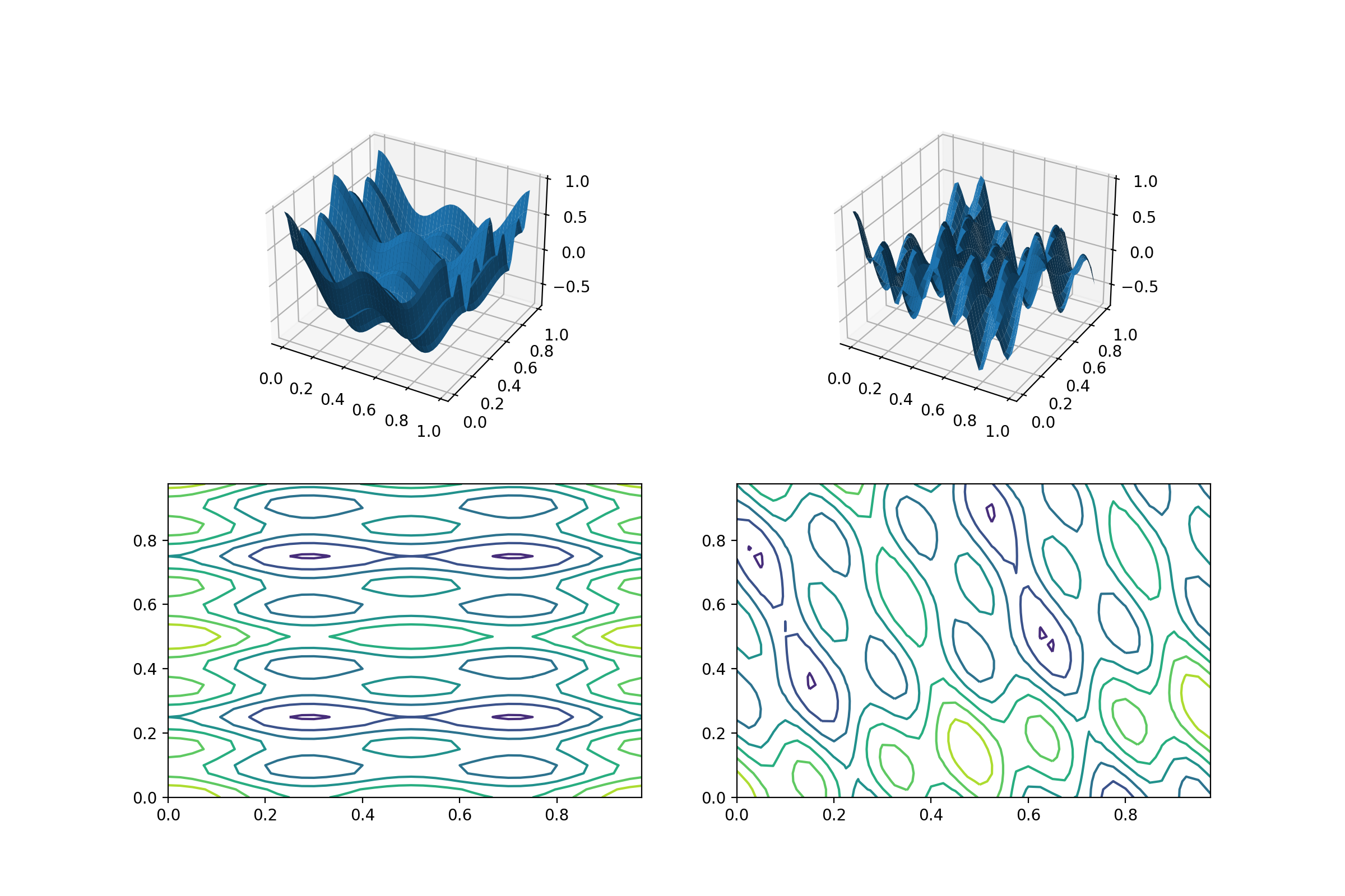
from matplotlib import pyplot as plt
from leap_ec.real_rep.problems import CosineFamilyProblem, MatrixTransformedProblem, plot_2d_problem

original_problem = CosineFamilyProblem(alpha=1.0, global_optima_counts=[2, 3], local_optima_counts=[2, 3])

transformed_problem = MatrixTransformedProblem.random_orthonormal(original_problem, 2)

fig = plt.figure(figsize=(12, 8))

plt.subplot(221, projection='3d')
bounds = original_problem.bounds
plot_2d_problem(original_problem, xlim=bounds, ylim=bounds, ax=plt.gca(), granularity=0.025)

plt.subplot(222, projection='3d')
plot_2d_problem(transformed_problem, xlim=bounds, ylim=bounds, ax=plt.gca(), granularity=0.025)

plt.subplot(223)
plot_2d_problem(original_problem, kind='contour', xlim=bounds, ylim=bounds, ax=plt.gca(), granularity=0.025)

plt.subplot(224)
plot_2d_problem(transformed_problem, kind='contour', xlim=bounds, ylim=bounds, ax=plt.gca(), granularity=0.025)

(Source code, png, hires.png, pdf)

class leap_ec.real_rep.problems.NoisyQuarticProblem(maximize=False)

The classic ‘quadratic quartic’ function with Gaussian noise:

\[f(\mathbf{x}) = \sum_{i=1}^{n} i x_i^4 + \texttt{gauss}(0, 1)\]

Parameters

maximize (bool) – the function is maximized if True, else minimized.

from leap_ec.real_rep.problems import NoisyQuarticProblem, plot_2d_problem
bounds = NoisyQuarticProblem.bounds  # Contains traditional bounds
plot_2d_problem(NoisyQuarticProblem(), xlim=bounds, ylim=bounds, granularity=0.025)

(Source code, png, hires.png, pdf)

bounds = (-1.28, 1.28)

evaluate(phenome)

Computes the function value from a real-valued list phenome (the output varies, since the function has noise):

>>> phenome = [3.5, -3.8, 5.0]
>>> r = NoisyQuarticProblem().evaluate(phenome)
>>> print(f'Result: {r}')
Result: ...

Parameters

phenome – real-valued vector to be evaluated

Returns

its fitness

worse_than(first_fitness, second_fitness)

We minimize by default:

>>> s = NoisyQuarticProblem()
>>> s.worse_than(100, 10)
True

>>> s = NoisyQuarticProblem(maximize=True)
>>> s.worse_than(100, 10)
False

class leap_ec.real_rep.problems.RastriginProblem(a=1.0, maximize=False)

The classic Rastrigin problem. The Rastrigin provides a real-valued fitness landscape with a quadratic global structure (like the SpheroidProblem), plus a sinusoidal local structure with many local optima.

\[f(\vec{x}) = An + \sum_{i=1}^n x_i^2 - A\cos(2\pi x_i)\]

Parameters

maximize (bool) – the function is maximized if True, else minimized.

from leap_ec.real_rep.problems import RastriginProblem, plot_2d_problem
bounds = RastriginProblem.bounds  # Contains traditional bounds
plot_2d_problem(RastriginProblem(), xlim=bounds, ylim=bounds, granularity=0.025)

(Source code, png, hires.png, pdf)

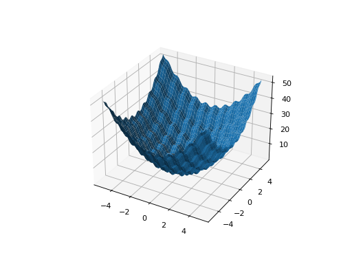
bounds = (-5.12, 5.12)

evaluate(phenome)

Computes the function value from a real-valued list phenome:

>>> phenome = [1.0/12, 0]
>>> RastriginProblem().evaluate(phenome) # +doctest: ELLIPSIS
0.1409190406...

Parameters

phenome – real-valued vector to be evaluated

Returns

its fitness

worse_than(first_fitness, second_fitness)

We minimize by default:

>>> s = NoisyQuarticProblem()
>>> s.worse_than(100, 10)
True

>>> s = NoisyQuarticProblem(maximize=True)
>>> s.worse_than(100, 10)
False

class leap_ec.real_rep.problems.RosenbrockProblem(maximize=False)

The classic RosenbrockProblem problem, a.k.a. the “banana” or “valley” function.

\[f(\mathbf{x}) = \sum_{i=1}^{d-1} \left[ 100 (x_{i + 1} - x_i^2)^2 + (x_i - 1)^2\right]\]

Parameters

maximize (bool) – the function is maximized if True, else minimized.

from leap_ec.real_rep.problems import RosenbrockProblem, plot_2d_problem
bounds = RosenbrockProblem.bounds  # Contains traditional bounds
plot_2d_problem(RosenbrockProblem(), xlim=bounds, ylim=bounds, granularity=0.025)

(Source code, png, hires.png, pdf)

bounds = (-2.048, 2.048)

evaluate(phenome)

Computes the function value from a real-valued list phenome:

>>> phenome = [0.5, -0.2, 0.1]
>>> RosenbrockProblem().evaluate(phenome)
22.3

Parameters

phenome – real-valued vector to be evaluated

Returns

its fitness

worse_than(first_fitness, second_fitness)

We minimize by default:

>>> s = NoisyQuarticProblem()
>>> s.worse_than(100, 10)
True

>>> s = NoisyQuarticProblem(maximize=True)
>>> s.worse_than(100, 10)
False

class leap_ec.real_rep.problems.ScaledProblem(problem, new_bounds, maximize=None)

Scale the search space of a fitness function up or down.

evaluate(phenome)

Decode and evaluate the given individual based on its genome.

Practitioners must over-ride this member function.

Note that by default the individual comparison operators assume a maximization problem; if this is a minimization problem, then just negate the value when returning the fitness.

Parameters

phenome –

Returns

fitness

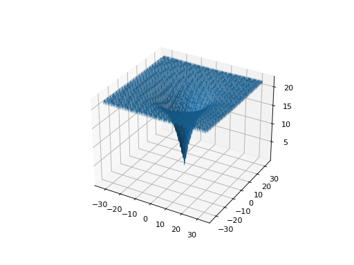
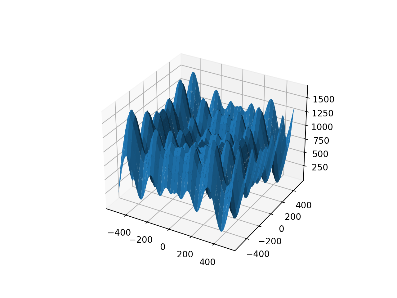
class leap_ec.real_rep.problems.SchwefelProblem(alpha=418.982887, maximize=False)

Schwefel’s function is another traditional multimodal test function whose local optima are distributed in a slightly irregular way, and whose global optimum is out at the edge of the search space (with no gently sloping macrostructure to guide the algorithm toward it).

Compare this to the RastriginProblem function, whose global optimum lies at the center of a quadratic bowl with a regular grid of local optima.

\[f(\mathbf{x}) = \sum_{i=1}^d\left(-x_i \cdot\sin\left(\sqrt{\|x_i\|} \right)\right) + \alpha \cdot d\]

Parameters

• alpha (float) – fitness offset (the default value ensures that the global optimum has zero fitness)

• maximize (bool) – the function is maximized if True, else minimized.

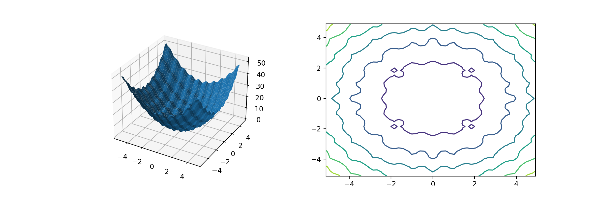
from leap_ec.real_rep.problems import SchwefelProblem, plot_2d_problem
bounds = SchwefelProblem.bounds  # Contains traditional bounds
plot_2d_problem(SchwefelProblem(), xlim=bounds, ylim=bounds, granularity=10)

(Source code, png, hires.png, pdf)

bounds = (-512, 512)

evaluate(phenome)

Computes the function value from a real-valued phenome.

Parameters

phenome – real-valued vector to be evaluated

Returns

its fitness.

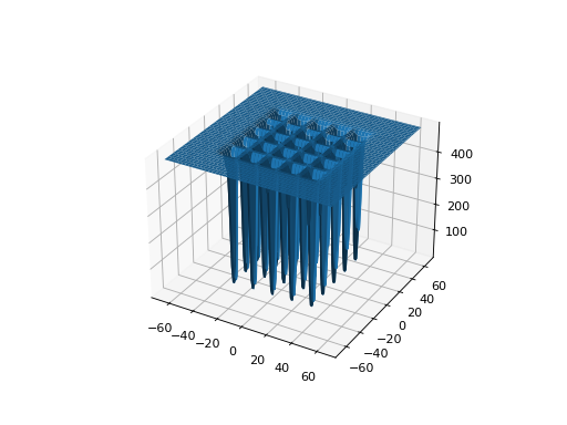
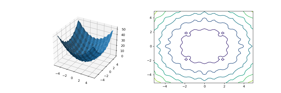
class leap_ec.real_rep.problems.ShekelProblem(k=500, c=array([1, 2, 3, 4, 5, 6, 7, 8, 9, 10, 11, 12, 13, 14, 15, 16, 17, 18, 19, 20, 21, 22, 23, 24, 25]), maximize=False)

The classic ‘Shekel’s foxholes’ function.

\[f(\mathbf{x}) = \frac{1}{\frac{1}{K} + \sum_{j=1}^{25} \frac{1}{f_j(\mathbf{x})}}\]

where

\[f_j(\mathbf{x}) = c_j + \sum_{i=1}^2 (x_i - a_{ij})^6\]

and the points \(\left\{ (a_{1j}, a_{2j})\right\}_{j=1}^{25}\) define the functions various optima, and are given by the following hardcoded matrix:

\[\begin{split}\left[a_{ij}\right] = \left[ \begin{array}{lllllllllll} -32 & -16 & 0 & 16 & 32 & -32 & -16 & \cdots & 0 & 16 & 32 \\ -32 & -32 & -32 & -32 & -32 & -16 & -16 & \cdots & 32 & 32 & 32 \end{array} \right].\end{split}\]

Parameters

• k (int) – the value of \(K\) in the fitness function.

• c ([int]) – list of values for the function’s \(c_j\) parameters. Each c[j] approximately corresponds to the depth of the jth foxhole.

• maximize (bool) – the function is maximized if True, else minimized.

• maximize – the function is maximized if True, else minimized.

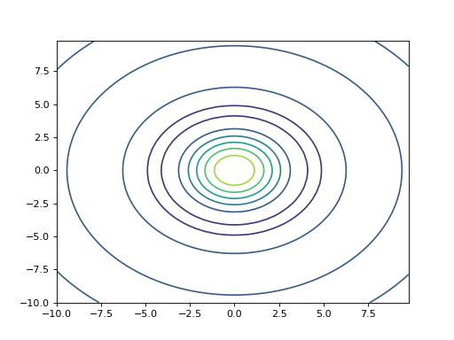
from leap_ec.real_rep.problems import ShekelProblem, plot_2d_problem
bounds = ShekelProblem.bounds  # Contains traditional bounds
plot_2d_problem(ShekelProblem(), xlim=bounds, ylim=bounds, granularity=0.9)

(Source code, png, hires.png, pdf)

bounds = (-65.536, 65.536)

evaluate(phenome)

Computes the function value from a real-valued list phenome (the output varies, since the function has noise).

Parameters

phenome – real-valued to be evaluated

Returns

its fitness

points = array([[-32, -16, 0, 16, 32, -32, -16, 0, 16, 32, -32, -16, 0, 16, 32, -32, -16, 0, 16, 32, -32, -16, 0, 16, 32], [-32, -32, -32, -32, -32, -16, -16, -16, -16, -16, 0, 0, 0, 0, 0, 16, 16, 16, 16, 16, 32, 32, 32, 32, 32]])

worse_than(first_fitness, second_fitness)

We minimize by default:

>>> s = ShekelProblem()
>>> s.worse_than(100, 10)
True

>>> s = ShekelProblem(maximize=True)
>>> s.worse_than(100, 10)
False

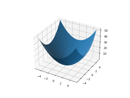
class leap_ec.real_rep.problems.SpheroidProblem(maximize=False)

Classic paraboloid function, known as the “sphere” or “spheroid” problem, because its equal-fitness contours form (hyper)spheres in n > 2.

\[f(\vec{x}) = \sum_{i}^n x_i^2\]

Parameters

maximize (bool) – the function is maximized if True, else minimized.

from leap_ec.real_rep.problems import SpheroidProblem, plot_2d_problem
bounds = SpheroidProblem.bounds  # Contains traditional bounds
plot_2d_problem(SpheroidProblem(), xlim=bounds, ylim=bounds, granularity=0.025)

(Source code, png, hires.png, pdf)

bounds = (-5.12, 5.12)

evaluate(phenome)

Computes the function value from a real-valued list phenome:

>>> phenome = [0.5, 0.8, 1.5]
>>> SpheroidProblem().evaluate(phenome)
3.14

Parameters

phenome – real-valued vector to be evaluated

Returns

it’s fitness, sum(phenome**2)

worse_than(first_fitness, second_fitness)

We minimize by default:

>>> s = NoisyQuarticProblem()
>>> s.worse_than(100, 10)
True

>>> s = NoisyQuarticProblem(maximize=True)
>>> s.worse_than(100, 10)
False

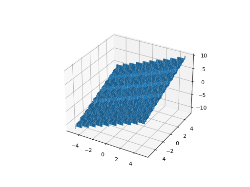
class leap_ec.real_rep.problems.StepProblem(maximize=True)

The classic ‘step’ function—a function with a linear global structure, but with stair-like plateaus at the local level.

\[f(\mathbf{x}) = \sum_{i=1}^{n} \lfloor x_i \rfloor\]

where \(\lfloor x \rfloor\) denotes the floor function.

Parameters

maximize (bool) – the function is maximized if True, else minimized.

from leap_ec.real_rep.problems import StepProblem, plot_2d_problem
bounds = StepProblem.bounds  # Contains traditional bounds
plot_2d_problem(StepProblem(), xlim=bounds, ylim=bounds, granularity=0.025)

(Source code, png, hires.png, pdf)

bounds = (-5.12, 5.12)

evaluate(phenome)

Computes the function value from a real-valued list phenome:

>>> phenome = [3.5, -3.8, 5.0]
>>> StepProblem().evaluate(phenome)
4.0

Parameters

phenome – real-valued vector to be evaluated

Returns

its fitness

worse_than(first_fitness, second_fitness)

We maximize by default:

>>> s = StepProblem()
>>> s.worse_than(100, 10)
False

>>> s = StepProblem(maximize=False)
>>> s.worse_than(100, 10)
True

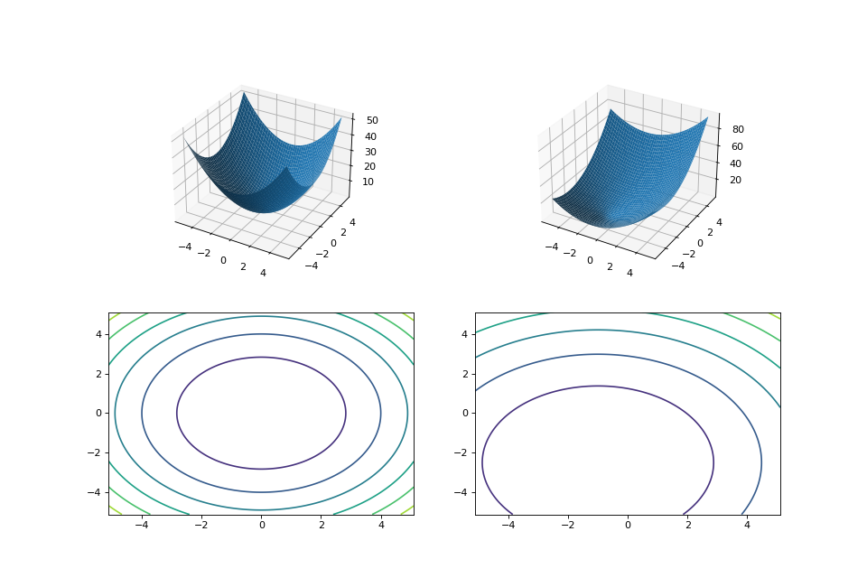
class leap_ec.real_rep.problems.TranslatedProblem(problem, offset, maximize=None)

Takes an existing fitness function and translates it by applying a fixed offset vector.

For example,

from matplotlib import pyplot as plt
from leap_ec.real_rep.problems import SpheroidProblem, TranslatedProblem, plot_2d_problem

original_problem = SpheroidProblem()
offset = [-1.0, -2.5]
translated_problem = TranslatedProblem(original_problem, offset)

fig = plt.figure(figsize=(12, 8))

plt.subplot(221, projection='3d')
bounds = SpheroidProblem.bounds  # Contains traditional bounds
plot_2d_problem(original_problem, xlim=bounds, ylim=bounds, ax=plt.gca(), granularity=0.025)

plt.subplot(222, projection='3d')
plot_2d_problem(translated_problem, xlim=bounds, ylim=bounds, ax=plt.gca(), granularity=0.025)

plt.subplot(223)
plot_2d_problem(original_problem, kind='contour', xlim=bounds, ylim=bounds, ax=plt.gca(), granularity=0.025)

plt.subplot(224)
plot_2d_problem(translated_problem, kind='contour', xlim=bounds, ylim=bounds, ax=plt.gca(), granularity=0.025)

(Source code, png, hires.png, pdf)

evaluate(phenome)

Evaluate the fitness of a point after translating the fitness function.

Translation can be used in higher than two dimensions:

>>> offset = [-1.0, -1.0, 1.0, 1.0, -5.0]
>>> t_sphere = TranslatedProblem(SpheroidProblem(), offset)
>>> genome = [0.5, 2.0, 3.0, 8.5, -0.6]
>>> t_sphere.evaluate(genome)
90.86

classmethod random(problem, offset_bounds, dimensions, maximize=None)

Apply a random real-valued translation to a fitness function, sampled uniformly between min_offset and max_offset in every dimension.

from leap_ec.real_rep.problems import RastriginProblem, plot_2d_problem

original_problem = RastriginProblem()
bounds = RastriginProblem.bounds  # Contains traditional bounds
translated_problem = TranslatedProblem.random(original_problem, bounds, 2)

plot_2d_problem(translated_problem, kind='contour', xlim=bounds, ylim=bounds)

(Source code)

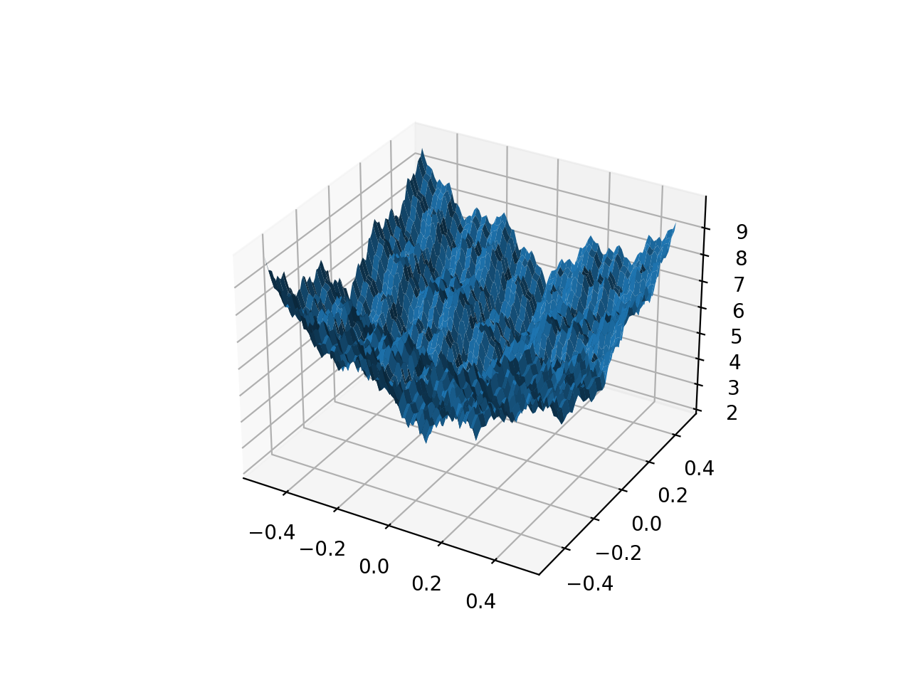
class leap_ec.real_rep.problems.WeierstrassProblem(kmax=20, a=0.5, b=3, maximize=False)

The Weierstrass function is famous for being the first discovered example of a function that is continuous, but not differentiable. Built by adding the terms of a Fourier series, it has a jagged, self-similar structure:

\[f(\mathbf{x}) = \sum_{i=1}^d \left[ \sum_{k=0}^{kmax} a^k \cos\left( 2\pi b^k(x_i + 0.5)\right) - n \sum_{k=0}^{kmax} a^k \cos(\pi b^k) \right]\]

When used in optimization benchmarks, it’s typical to carry out the Fourier sum to kmax=20 terms.

Parameters

• kmax (int) – number of terms to carry the Fourier sum out to

• a (float) – amplitude parameter of the cosine terms

• b (float) – wavenumber (frequency) parameter of the cosine terms

• maximize (bool) – the function is maximized if True, else minimized.

from leap_ec.real_rep.problems import WeierstrassProblem, plot_2d_problem
bounds = WeierstrassProblem.bounds  # Contains traditional bounds
plot_2d_problem(WeierstrassProblem(), xlim=bounds, ylim=bounds, granularity=0.01)

(Source code, png, hires.png, pdf)

bounds = [-0.5, 0.5]

evaluate(phenome)

Computes the function value from a real-valued phenome.

Parameters

phenome – real-valued vector to be evaluated

Returns

its fitness.

leap_ec.real_rep.problems.plot_2d_contour(fun, xlim, ylim, granularity, ax=None)

Convenience method for plotting contours for a function that accepts 2-D real-valued inputs and produces a 1-D scalar output.

Parameters

• fun (function) – The function to plot.

• xlim ((float, float)) – Bounds of the horizontal axes.

• ylim ((float, float)) – Bounds of the vertical axis.

• ax (Axes) – Matplotlib axes to plot to (if None, a new figure will be created).

• granularity (float) – Spacing of the grid to sample points along.

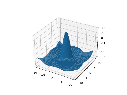
The difference between this and plot_2d_problem() is that this takes a raw function (instead of a Problem object).

import numpy as np
from scipy import linalg

from leap_ec.real_rep.problems import plot_2d_contour

def sinc_hd(phenome):
    r = linalg.norm(phenome)
    return np.sin(r)/r

plot_2d_contour(sinc_hd, xlim=(-10, 10), ylim=(-10, 10), granularity=0.2)

(Source code, png, hires.png, pdf)

leap_ec.real_rep.problems.plot_2d_function(fun, xlim, ylim, granularity=0.1, ax=None)

Convenience method for plotting a function that accepts 2-D real-valued imputs and produces a 1-D scalar output.

Parameters

• fun (function) – The function to plot.

• xlim ((float, float)) – Bounds of the horizontal axes.

• ylim ((float, float)) – Bounds of the vertical axis.

• ax (Axes) – Matplotlib axes to plot to (if None, a new figure will be created).

• granularity (float) – Spacing of the grid to sample points along.

The difference between this and plot_2d_problem() is that this takes a raw function (instead of a Problem object).

import numpy as np
from scipy import linalg

from leap_ec.real_rep.problems import plot_2d_function

def sinc_hd(phenome):
    r = linalg.norm(phenome)
    return np.sin(r)/r

plot_2d_function(sinc_hd, xlim=(-10, 10), ylim=(-10, 10), granularity=0.2)

(Source code, png, hires.png, pdf)

leap_ec.real_rep.problems.plot_2d_problem(problem, xlim, ylim, kind='surface', ax=None, granularity=None)

Convenience function for plotting a Problem that accepts 2-D real-valued phenomes and produces a 1-D scalar fitness output.

Parameters

• fun (Problem) – The Problem to plot.

• xlim ((float, float)) – Bounds of the horizontal axes.

• ylim ((float, float)) – Bounds of the vertical axis.

• kind (str) – The kind of plot to create: ‘surface’ or ‘contour’

• ax (Axes) – Matplotlib axes to plot to (if None, a new figure will be created).

• granularity (float) – Spacing of the grid to sample points along. If none is given, then the granularity will default to 1/50th of the range of the function’s bounds attribute.

The difference between this and plot_2d_function() is that this takes a Problem object (instead of a raw function).

If no axes are specified, a new figure is created for the plot:

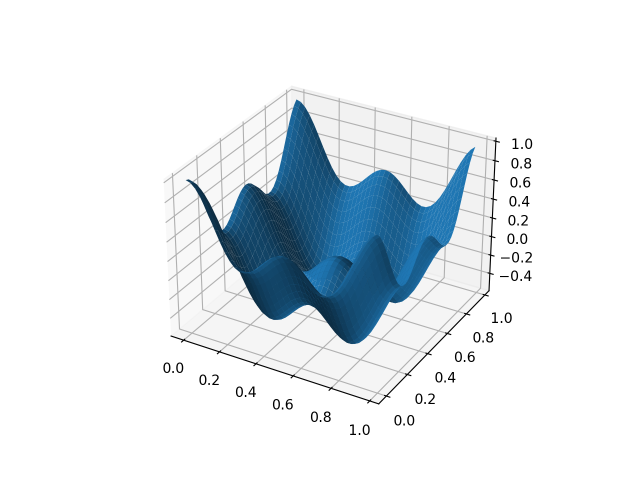
from leap_ec.real_rep.problems import CosineFamilyProblem, plot_2d_problem
problem = CosineFamilyProblem(alpha=1.0, global_optima_counts=[2, 2], local_optima_counts=[2, 2])
plot_2d_problem(problem, xlim=(0, 1), ylim=(0, 1), granularity=0.025);

(Source code, png, hires.png, pdf)

You can also specify axes explicitly (ex. by using ax=plt.gca(). When plotting surfaces, you must configure your axes to use projection=’3d’. Contour plots don’t need 3D axes:

from matplotlib import pyplot as plt
from leap_ec.real_rep.problems import RastriginProblem, plot_2d_problem

fig = plt.figure(figsize=(12, 4))
bounds=RastriginProblem.bounds  # Contains default bounds

plt.subplot(121, projection='3d')
plot_2d_problem(RastriginProblem(), ax=plt.gca(), xlim=bounds, ylim=bounds)

plt.subplot(122)
plot_2d_problem(RastriginProblem(), ax=plt.gca(), kind='contour', xlim=bounds, ylim=bounds)

(Source code, png, hires.png, pdf)