Distributed LEAP

LEAP supports synchronous and asynchronous distributed concurrent fitness evaluations that can significantly speed-up runs. LEAP uses dask (https://dask.org/), which is a popular distributed processing python package, to implement parallel fitness evaluations, and which allows easy scaling from laptops to supercomputers.

Synchronous fitness evaluations

Synchronous fitness evaluations are essentially a map/reduce approach where individuals are fanned out to computing resources to be concurrently evaluated, and then the calling process waits until all the evaluations are done. This is particularly suited for by-generation approaches where offspring are evaluated in a batch, and progress in the EA only proceeds when all individuals have been evaluated.

Components

leap_ec.distrib.synchronous provides two components to implement synchronous individual parallel evaluations.

leap_ec.distrib.synchronous.eval_population

which evaluates an entire population in parallel, and returns the evaluated population

leap_ec.distrib.synchronous.eval_pool

is a pipeline operator that will collect offspring and then evaluate them all at once in parallel; the evaluated offspring are returned

Example

The following shows a simple example of how to use the synchronous parallel fitness evaluation in LEAP.

#!/usr/bin/env python
""" Simple example of using leap_ec.distrib.synchronous

"""
import os

from distributed import Client
import toolz

from leap_ec import context, test_env_var
from leap_ec import ops
from leap_ec.decoder import IdentityDecoder
from leap_ec.binary_rep.initializers import create_binary_sequence
from leap_ec.binary_rep.ops import mutate_bitflip
from leap_ec.binary_rep.problems import MaxOnes
from leap_ec.distrib import DistributedIndividual
from leap_ec.distrib import synchronous
from leap_ec.probe import AttributesCSVProbe


##############################
# Entry point
##############################
if __name__ == '__main__':

    # We've added some additional state to the probe for DistributedIndividual,
    # so we want to capture that.
    probe = AttributesCSVProbe(attributes=['hostname',
                                           'pid',
                                           'uuid',
                                           'birth_id',
                                           'start_eval_time',
                                           'stop_eval_time'],
                               do_fitness=True,
                               do_genome=True,
                               stream=open('simple_sync_distributed.csv', 'w'))

    # Just to demonstrate multiple outputs, we'll have a separate probe that
    # will take snapshots of the offspring before culling.  That way we can
    # compare the before and after to see what specific individuals were culled.
    offspring_probe = AttributesCSVProbe(attributes=['hostname',
                                           'pid',
                                           'uuid',
                                           'birth_id',
                                           'start_eval_time',
                                           'stop_eval_time'],
                               do_fitness=True,
                               stream=open('simple_sync_distributed_offspring.csv', 'w'))

    with Client() as client:
        # create an initial population of 5 parents of 4 bits each for the
        # MAX ONES problem
        parents = DistributedIndividual.create_population(5, # make five individuals
                                                          initialize=create_binary_sequence(
                                                              4), # with four bits
                                                          decoder=IdentityDecoder(),
                                                          problem=MaxOnes())

        # Scatter the initial parents to dask workers for evaluation
        parents = synchronous.eval_population(parents, client=client)

        # probes rely on this information for printing CSV 'step' column
        context['leap']['generation'] = 0

        probe(parents) # generation 0 is initial population
        offspring_probe(parents) # generation 0 is initial population

        # When running the test harness, just run for two generations
        # (we use this to quickly ensure our examples don't get bitrot)
        if os.environ.get(test_env_var, False) == 'True':
            generations = 2
        else:
            generations = 5

        for current_generation in range(generations):
            context['leap']['generation'] += 1

            offspring = toolz.pipe(parents,
                                   ops.tournament_selection,
                                   ops.clone,
                                   mutate_bitflip(expected_num_mutations=1),
                                   ops.UniformCrossover(),
                                   # Scatter offspring to be evaluated
                                   synchronous.eval_pool(client=client,
                                                         size=len(parents)),
                                   offspring_probe, # snapshot before culling
                                   ops.elitist_survival(parents=parents),
                                   # snapshot of population after culling
                                   # in separate CSV file
                                   probe)

            print('generation:', current_generation)
            [print(x.genome, x.fitness) for x in offspring]

            parents = offspring

    print('Final population:')
    [print(x.genome, x.fitness) for x in parents]

This example of a basic genetic algorithm that solves the MAX ONES problem does not use a provided monolithic entry point, such as found with ea_solve() or generational_ea() but, instead, directly uses LEAP’s pipeline architecture. Here, we create a simple dask Client that uses the default local cores to do the parallel evaluations. The first step is to create the initial random population, and then distribute those to dask workers for evaluation via synchronous.eval_population(), and which returns a set of fully evaluated parents. The for loop supports the number of generations we want, and provides a sequence of pipeline operators to create offspring from selected parents. For concurrently evaluating newly created offspring, we use synchronous.eval_pool, which is just a variant of the leap_ec.ops.pool operator that relies on dask to evaluate individuals in parallel.

Note

If you wanted to use resources on a cluster or supercomputer, you would start up dask-scheduler and dask-worker`s first, and then point the `Client at the scheduler file used by the scheduler and workers. Distributed LEAP is agnostic on what kind of dask client is passed as a client parameter – it will generically perform the same whether running on local cores or on a supercomputer.

Separate Examples

There is a jupyter notebook that walks through a synchronous implementation in examples/distributed/simple_sync_distributed.ipynb. The above example can also be found at examples/distributed/simple_sync_distributed.py.

Asynchronous fitness evaluations

Asynchronous fitness evaluations are a little more involved in that the EA immediately integrates newly evaluated individuals into the population – it doesn’t wait until all the individuals have finished evaluating before proceeding. More specifically, LEAP implements an asynchronous steady-state evolutionary algorithm (ASEA).

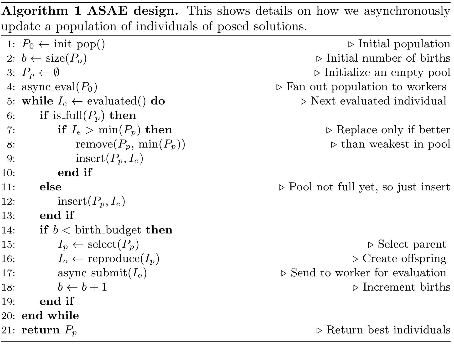
Fig. 10 Algorithm 1: Asynchronous steady-state evolutionary algorithm concurrently updates a population as individuals are evaluated [CSB20].

Algorithm 1 shows the details of how an ASEA works. Newly evaluated individuals are inserted into the population, which then leaves a computing resource available. Offspring are created from one or more selected parents, and are then assigned to that computing resource, thus assuring minimal idle time between evaluations. This is particularly important within HPC contexts as it is often the case that such resources are costly, and therefore there is an implicit need to minimize wasting such resources. By contrast, a synchronous distributed approach risks wasting computing resources because computing resources that finish evaluating individuals before the last individual is evaluated will idle until the next generation.

Example

from pprint import pformat

from dask.distributed import Client, LocalCluster

from leap_ec import Representation
from leap_ec import ops
from leap_ec.binary_rep.problems import MaxOnes
from leap_ec.binary_rep.initializers import create_binary_sequence
from leap_ec.binary_rep.ops import mutate_bitflip
from leap_ec.distrib import DistributedIndividual
from leap_ec.distrib import asynchronous
from leap_ec.distrib.probe import log_worker_location, log_pop

MAX_BIRTHS = 500
INIT_POP_SIZE = 20
POP_SIZE = 20
GENOME_LENGTH = 5

with Client(scheduler_file='scheduler.json') as client:
    final_pop = asynchronous.steady_state(client, # dask client
                                  births=MAX_BIRTHS,
                                  init_pop_size=INIT_POP_SIZE,
                                  pop_size=POP_SIZE,

                                  representation=Representation(
                                      initialize=create_binary_sequence(
                                          GENOME_LENGTH),
                                      individual_cls=DistributedIndividual),

                                  problem=MaxOnes(),

                                  offspring_pipeline=[
                                      ops.random_selection,
                                      ops.clone,
                                          mutate_bitflip,
                                      ops.pool(size=1)],

                                  evaluated_probe=track_workers_func,
                                  pop_probe=track_pop_func)

print(f'Final pop: \n{pformat(final_pop)}')

The above example is quite different from the synchronous code given earlier. Unlike, with the synchronous code, the asynchronous code does provide a monolithic function entry point, asynchronous.steady_state(). The first thing to note is that by nature this EA has a birth budget, not a generation budget, and which is set to 500 in MAX_BIRTHS, and passed in via the births parameter. We also need to know the size of the initial population, which is given in init_pop_size. And, of course, we need the size of the population that is perpetually updated during the lifetime of the run, and which is passed in via the pop_size parameter.

The representation parameter we have seen before in the other monolithic functions, such as generational_ea, which encapsulates the mechanisms for making an individual and how the individual’s state is stored. In this case, because it’s the MAX ONES problem, we use the IdentityDecoder because we want to use the raw bits as is, and we specify a factory function for creating binary sequences GENOME_LENGTH in size; and, lastly, we override the default class with a new class, DistributedIndividual, that contains some additional bookkeeping useful for an ASEA, and is described later.

The offspring_pipeline differs from the usual LEAP pipelines. That is, a LEAP pipeline is usally a set of operators that define a workflow for creating offspring from a set of prospective parents. In this case, the pipeline is for creating a single offspring from an implied population of prospective parents to be evaluated on a recently available dask worker; essentially, as a dask worker finishes evaluating an individual, this pipeline will be used to create a single offspring to be assigned to that worker for evaluation. This gives the user maximum flexibility in how that offspring is created by choosing a selection operator followed by perturbation operators deemed suitable for the given problem. (Not forgetting the critical clone operator, the absence of which will cause selected parents to be modified by any applied mutation or crossover operators.)

There are two optional callback function reporting parameters, evaluated_probe and pop_probe. evaluated_probe takes a single Individual class, or subclass, as an argument, and can be used to write out that individual’s state in a desired format. distrib.probe.log_worker_location can be passed in as this argument to write each individual’s state as a CSV row to a file; by default it will write to sys.stdout. The pop_probe parameter is similar, but allows for taking snapshots of the hidden population at preset intervals, also in CSV format.

Also noteworthy is that the Client has a scheduler_file specified, which indicates that a dask scheduler and one or more dask workers have already been started beforehand outside of LEAP and are awaiting tasking to evaluate individuals.

There are three other optional parameters to steady_state, which are summarized as follows:

inserter

takes a callback function of the signature (individual, population, max_size) where individual is the newly evaluated individual that is a candidate for inserting into the population, and which is the internal population that steady_state updates. The value for max_size is passed in by steady_state that is the user stipulated population size, and is used to determine if the individual should just be inserted into the population when at the start of the run it has yet to reach capacity. That is, when a user invokes steady_state, they specify a population size via pop_size, and we would just normally insert individuals until the population reaches pop_size in capacity, then the function will use criteria to determine whether the individual is worthy of being inserted. (And, if so, at the removal of an individual that was already in the population. Or, colloquially, someone is voted off the island.)

There are two provided inserters, steady_state.tournament_insert_into_pop and greedy_insert_into_pop. The first will randomly select an individual from the internal population, and will replace it if its fitness is worse than the new individual. The second will compare the new individual with the current worst in the population, and will replace that individual if it is better. The default for inserter is to use the greedy_insert_into_pop.

Of course you can write your own if either of these two inserters do not meet your needs.

count_nonviable

is a boolean that, if True, means that individuals that are non- viable are counted towards the birth budget; by default, this is False. A non-viable individual is one where an exception was thrown during evaluation. (E.g., an individual poses a deep-learner configuration that does not make sense, such as incompatible adjacent convolutional layers, and pytorch or tensorflow throws an exception.)

context

contains global state where the running number of births and non-viable individuals is kept. This defaults to context.

DistributedIndividual

DistributedIndividual is a subclass of RobustIndividual that contains some additional state that may be useful for distributed fitness evaluations.

uuid

is UUID assigned to that individual upon creation

birth_id

is a unique, monotonically increasing integer assigned to each indidividual on creation, and denotes its birth order

start_eval_time

is when evaluation began for this individul, and is in time_t format

stop_eval_time

when evaluation completed in time_t format

This additional state is set in distrib.evaluate.evaluate() and is_viable and exception are set as with the base class, core.Individual.

Note

The uuid is useful if one wanted to save, say, a model or some other state in a file; using the uuid in the file name will make it easier to associate the file with a given individual later during a run’s post mortem analysis.

Note

The start_eval_time and end_eval_time can be useful for checking whether individuals that take less time to evaluate come to dominate the population, which can be important in ASEA parameter tuning. E.g., initially the population will come to be dominated by individuals that evaluated quickly even if they represent inferior solutions; however, eventually, better solutions that take longer to evaluate will come to dominate the population; so, if one observes that shorter solutions still dominate the population, then increasing the max_births should be considered, if feasible, to allow time for solutions that need longer to evaluate time to make a representative presence in the population.

Separate Examples

There is also a jupyter notebook walkthrough for the asynchronous implementation, examples/distributed/simple_async_distributed.ipynb. Moreover, there is standalone code in examples/distributed/simple_async_distributed.py.