leap_ec.real_rep package
Submodules
leap_ec.real_rep.initializers module
Initializers for real values.
- leap_ec.real_rep.initializers.create_real_vector(bounds)
A closure for initializing lists of real numbers for real-valued genomes, sampled from a uniform distribution.
Having a closure allows us to just call the returned function N times in Individual.create_population().
TODO Allow either a single tuple or a test_sequence of tuples for bounds. —Siggy
- Parameters
bounds – a list of (min, max) values bounding the uniform sampline of each element
- Returns
A function that, when called, generates a random genome.
E.g., can be used for Individual.create_population()
>>> from leap_ec.decoder import IdentityDecoder
>>> from . problems import SpheroidProblem
>>> bounds = [(0, 1), (0, 1), (-1, 100)]
>>> population = Individual.create_population(10, create_real_vector(bounds),
...                                           decoder=IdentityDecoder(),
...                                           problem=SpheroidProblem())
leap_ec.real_rep.ops module
Pipeline operators for real-valued representations
- leap_ec.real_rep.ops.apply_hard_bounds(genome, hard_bounds)
A helper that ensures that every gene is contained within the given bounds.
- Parameters
genome – list of values to apply bounds to.
hard_bounds – if a (low, high) tuple, the same bounds will be used for every gene. If a list of tuples is given, then the ith bounds will be applied to the ith gene.
Both sides of the range are inclusive:
>>> genome = np.array([0, 10, 20, 30, 40, 50])
>>> apply_hard_bounds(genome, hard_bounds=(20, 40))
array([20, 20, 20, 30, 40, 40])
Different bounds can be used for each locus by passing in a list of tuples:
>>> bounds= [ (0, 1), (0, 1), (50, 100), (50, 100), (0, 100), (0, 10) ]
>>> apply_hard_bounds(genome, hard_bounds=bounds)
array([ 0,  1, 50, 50, 40, 10])
- leap_ec.real_rep.ops.genome_mutate_gaussian(genome='__no__default__', std: float = '__no__default__', expected_num_mutations='__no__default__', bounds: Tuple[float, float] = (-inf, inf), transform_slope: float = 1.0, transform_intercept: float = 0.0)
Perform Gaussian mutation directly on real-valued genes (rather than on an Individual).
This used to be inside mutate_gaussian, but was moved outside it so that leap_ec.segmented.ops.apply_mutation could directly use this function, thus saving us from doing a copy-n-paste of the same code to the segmented sub-package.
- Parameters
genome – of real-valued numbers that will potentially be mutated
std – the mutation width—either a single float that will be used for all genes, or a list of floats specifying the mutation width for each gene individually.
expected_num_mutations – on average how many mutations are expected
- Returns
mutated genome
- leap_ec.real_rep.ops.mutate_gaussian(next_individual: Iterator = '__no__default__', std='__no__default__', expected_num_mutations: Union[int, str] = None, bounds=(-inf, inf), transform_slope: float = 1.0, transform_intercept: float = 0.0) Iterator
Mutate and return an Individual with a real-valued representation.
This operators on an iterator of Individuals:
>>> from leap_ec.individual import Individual
>>> from leap_ec.real_rep.ops import mutate_gaussian
>>> import numpy as np
>>> pop = iter([Individual(np.array([1.0, 0.0]))])
Mutation can either use the same parameters for all genes:
>>> op = mutate_gaussian(std=1.0, expected_num_mutations='isotropic', bounds=(-5, 5))
>>> mutated = next(op(pop))
Or we can specify the std and bounds independently for each gene:
>>> pop = iter([Individual(np.array([1.0, 0.0]))])
>>> op = mutate_gaussian(std=[0.5, 1.0],
...                      expected_num_mutations='isotropic',
...                      bounds=[(-1, 1), (-10, 10)]
... )
>>> mutated = next(op(pop))
- Parameters
next_individual – to be mutated
std – standard deviation to be equally applied to all individuals; this can be a scalar value or a “shadow vector” of standard deviations
expected_num_mutations – if an int, the expected number of mutations per individual, on average. If ‘isotropic’, all genes will be mutated.
bounds – to clip for mutations; defaults to (- ∞, ∞)
- Returns
a generator of mutated individuals.
leap_ec.real_rep.problems module
This module contains a variety of classic real-valued optimization problems that frequently occur in research benchmarks.
It also contains helpers for translating, rotating, and visualizing them.
- class leap_ec.real_rep.problems.AckleyProblem(a=20, b=0.2, c=6.283185307179586, maximize=False)
Bases:
ScalarProblem\[f(\mathbf{x}) = -a \exp \left( -b \sqrt {\frac{1}{d} \sum_{i=1}^d x_i^2} \right) - \exp \left( \frac{1}{d} \sum_{i=1}^d \cos(cx_i) \right) + a + \exp(1)\]- Parameters
a (float) – depth parameter for the bowl-shaped macrostructure
b (float) – exponential scale parameter for the bowl
c (float) – wavenumber (frequency) of the cosine pattern of local optima
maximize (bool) – the function is maximized if True, else minimized.
from leap_ec.real_rep.problems import AckleyProblem, plot_2d_problem
import math
problem = AckleyProblem(a=20, b=0.2, c=2*math.pi)
bounds = AckleyProblem.bounds  # Contains traditional bounds
plot_2d_problem(problem, xlim=bounds, ylim=bounds, granularity=0.25)
(Source code, png, hires.png, pdf)

- bounds = [-32.768, 32.768]
- evaluate(phenome)
Computes the function value from a real-valued phenome.
- Parameters
phenome – real-valued vector to be evaluated
- Returns
its fitness.
- class leap_ec.real_rep.problems.CosineFamilyProblem(alpha, global_optima_counts, local_optima_counts, maximize=False)
Bases:
ScalarProblemA configurable multi-modal function based on combinations of cosines, taken from the problem generators proposed by Rönkkönen et al. [RonkkonenLKL08].
\[f_{\cos}(\mathbf{x}) = \frac{\sum_{i=1}^n -\cos((G_i - 1)2 \pi x_i) - \alpha \cdot \cos((G_i - 1)2 \pi L_i x_i)}{2n}\]where \(G_i\) and \(L_i\) are parameters that indicate the number of global and local optima, respectively, in the ith dimension.
- Parameters
alpha (float) – parameter that controls the depth of the local optima.
global_optima_counts ([int]) – list of integers indicating the number of global optima for each dimension.
local_optima_counts ([int]) – list of integers indicated the number of local optima for each dimension.
maximize – the function is maximized if True, else minimized.
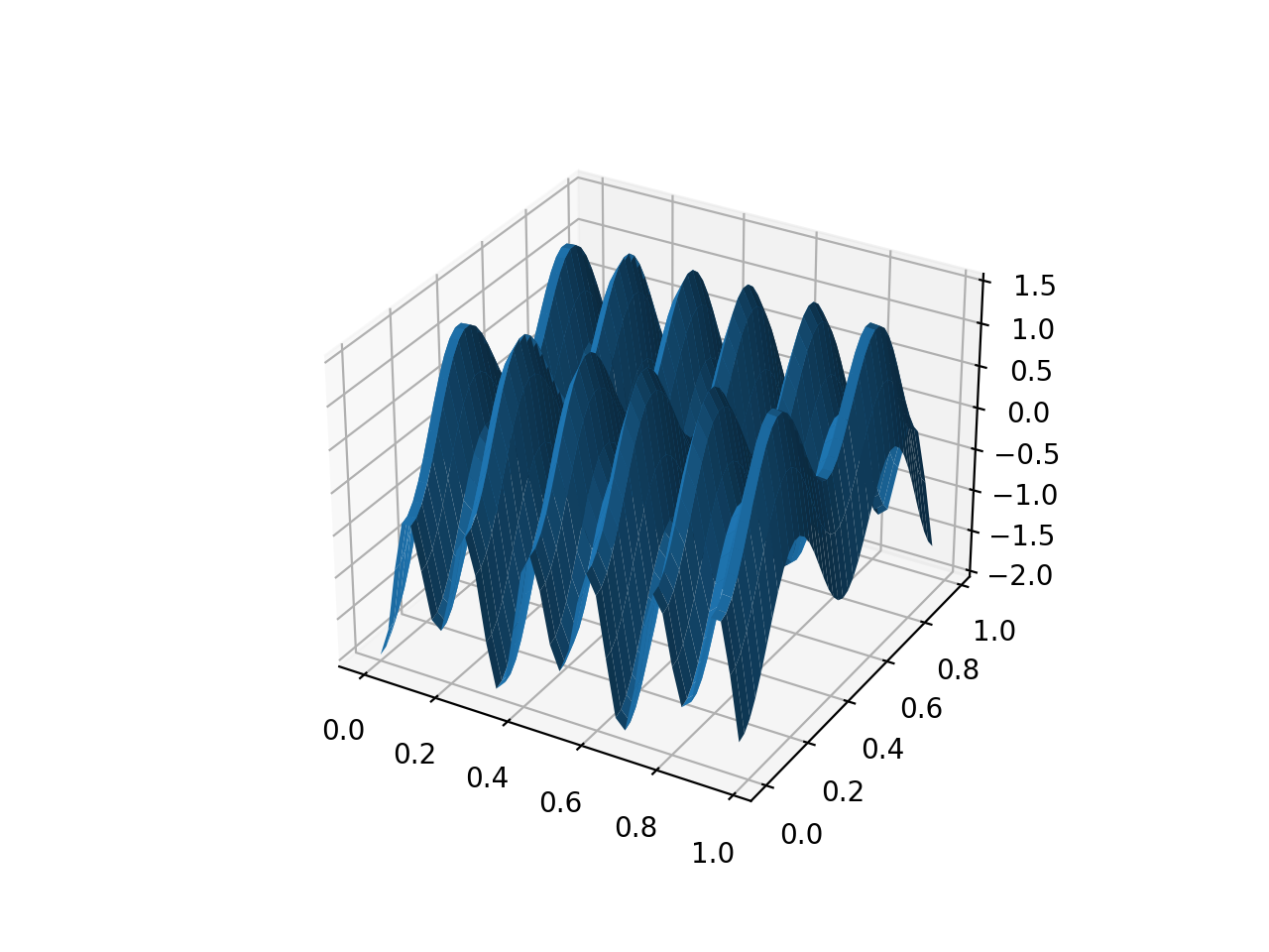
from leap_ec.real_rep.problems import CosineFamilyProblem, plot_2d_problem
problem = CosineFamilyProblem(alpha=1.0, global_optima_counts=[2, 2], local_optima_counts=[2, 2])
bounds = CosineFamilyProblem.bounds  # Contains traditional bounds
plot_2d_problem(problem, xlim=bounds, ylim=bounds, granularity=0.025)
(Source code, png, hires.png, pdf)

The number of optima can be varied independently by each dimension:
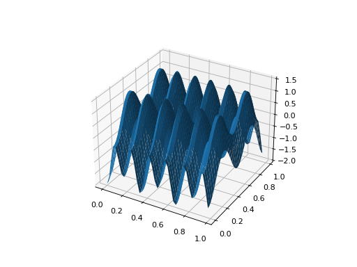
from leap_ec.real_rep.problems import CosineFamilyProblem, plot_2d_problem
problem = CosineFamilyProblem(alpha=3.0, global_optima_counts=[4, 2], local_optima_counts=[2, 2])
bounds = CosineFamilyProblem.bounds  # Contains traditional bounds
plot_2d_problem(problem, xlim=bounds, ylim=bounds, granularity=0.025)
(Source code, png, hires.png, pdf)

- bounds = (0, 1)
- evaluate(phenome)
Computes the function value from a real-valued phenome.
- Parameters
phenome – phenome with a real-valued phenome vector to be evaluated
- Returns
its fitness.
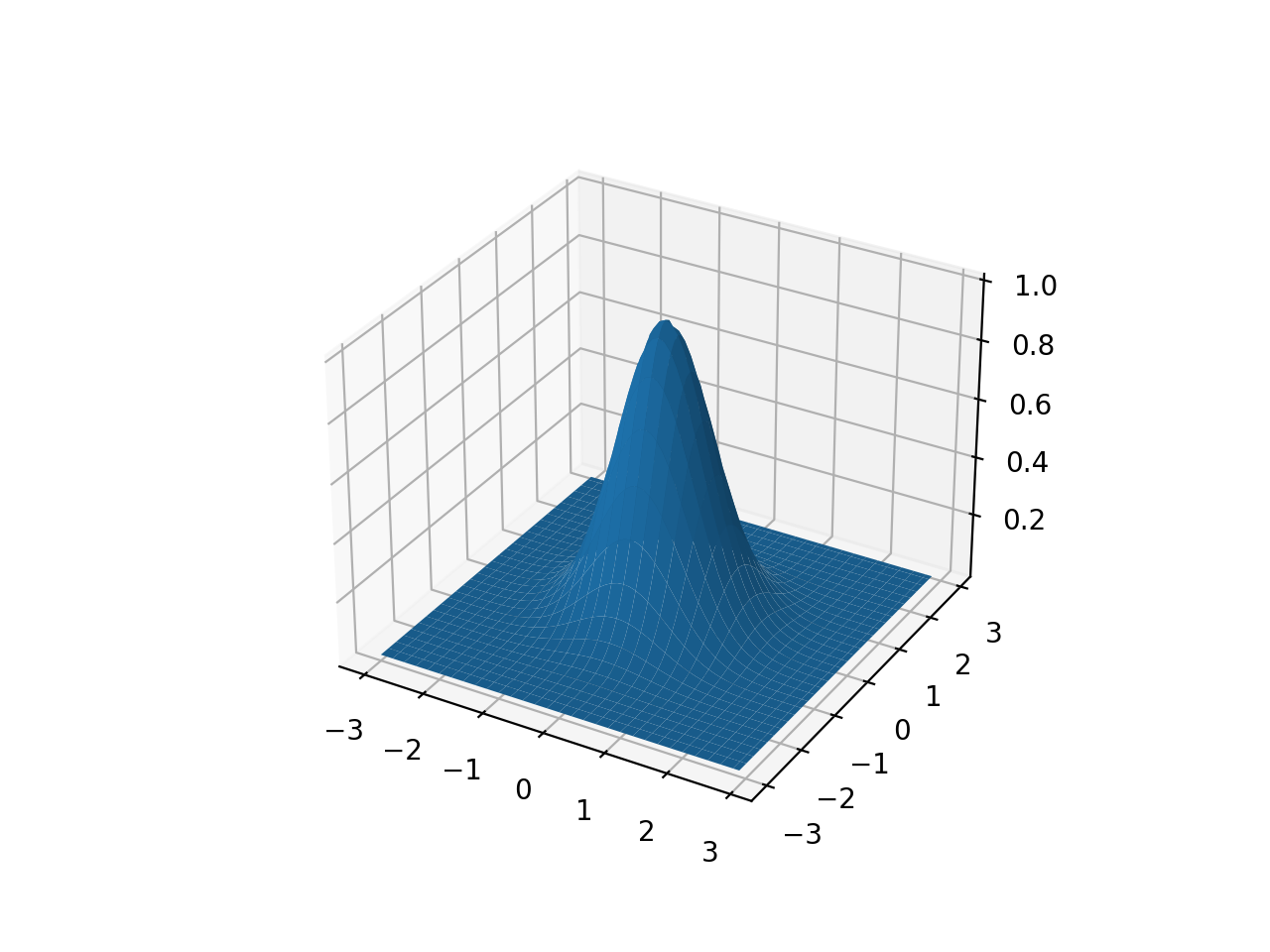
- class leap_ec.real_rep.problems.GaussianProblem(width=1, height=1, maximize=True)
Bases:
ScalarProblemA multidimensional, isotropic Gaussian function, defined by
\[A\exp\left( - \sum_i^n \left(\frac{x_i}{w}\right)^2 \right)\]- Parameters
width (float) – the width parameter \(w\)
height (float) – the height parameter \(A\)
from leap_ec.real_rep.problems import GaussianProblem, plot_2d_problem
bounds = GaussianProblem.bounds  # Some typical bounds
problem = GaussianProblem(width=1, height=1)
plot_2d_problem(problem, xlim=bounds, ylim=bounds, granularity=0.1)
(Source code, png, hires.png, pdf)

- bounds = (-3, 3)
- evaluate(phenome)
Evaluate the given phenome.
Practitioners must over-ride this member function.
Note that by default the individual comparison operators assume a maximization problem; if this is a minimization problem, then just negate the value when returning the fitness.
- Parameters
phenome – the phenome to evaluate (this will not be modified)
- Returns
the fitness value
- class leap_ec.real_rep.problems.GriewankProblem(maximize=False)
Bases:
ScalarProblemThe classic Griewank problem. Like the
RastriginProblemfunction, the Griewank has a quadratic global structure with many local optima that are distrib in a regular pattern.\[f(\mathbf{x}) = \sum_{i=1}^d \frac{x_i^2}{4000} - \prod_{i=1}^d \cos\left(\frac{x_i}{\sqrt{i}}\right) + 1\]- Parameters
maximize (bool) – the function is maximized if True, else minimized.
from leap_ec.real_rep.problems import GriewankProblem, plot_2d_problem
bounds = GriewankProblem.bounds  # Contains traditional bounds
plot_2d_problem(GriewankProblem(), xlim=bounds, ylim=bounds, granularity=10)
(Source code, png, hires.png, pdf)
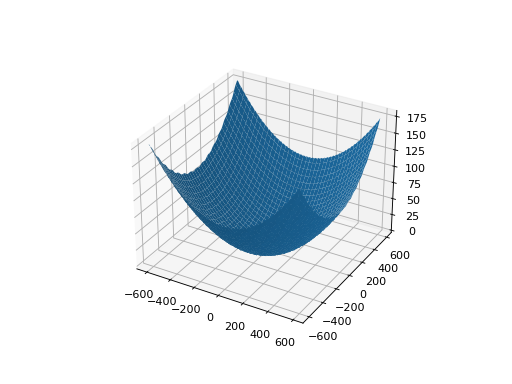
from leap_ec.real_rep.problems import GriewankProblem, plot_2d_problem
bounds = [-50, 50]
plot_2d_problem(GriewankProblem(), xlim=bounds, ylim=bounds, granularity=1)
(Source code, png, hires.png, pdf)
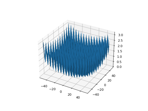
- bounds = [-600, 600]
- evaluate(phenome)
Computes the function value from a real-valued phenome.
- Parameters
phenome – real-valued vector to be evaluated
- Returns
its fitness.
- class leap_ec.real_rep.problems.LangermannProblem(m=5, c=(1, 2, 5, 2, 3), a=((3, 5), (5, 2), (2, 1), (1, 4), (7, 9)), maximize=False)
Bases:
ScalarProblemA popular multi-modal test function built by summing together \(m\) terms.
\[f(\mathbf{x}) = -\sum_{i=1}^m c_i \exp\left( -\frac{1}{\pi} \sum_{j=1}^d(x_j - A_{ij})^2\right) \cos\left(\pi\sum_{j=1}^d(x_j - A_{ij})^2\right)\]Langermann’s function is parameterized by a vector \(c_i\) of length \(m\) and a matrix \(A_{ij}\) of dimension \(m \times d\). This class uses the traditional parameterization as the default, with \(m=5\) and
\[\begin{split}c = (1, 2, 5, 2, 3) \\ A = \left[ \begin{array}{ll} 3 & 5\\ 5 & 2\\ 2 & 1\\ 1 & 4\\ 7 & 9 \end{array} \right].\end{split}\]- Parameters
m (int) – total number of terms in the function’s sum
c ([float]) – amplitude coefficients for each term
a ([[float]]) – offsets points for each term
maximize (bool) – the function is maximized if True, else minimized.
from leap_ec.real_rep.problems import LangermannProblem, plot_2d_problem
bounds = LangermannProblem.bounds  # Contains traditional bounds
plot_2d_problem(LangermannProblem(), xlim=bounds, ylim=bounds, granularity=0.2)
(Source code, png, hires.png, pdf)

- bounds = [0, 10]
- default_a = ((3, 5), (5, 2), (2, 1), (1, 4), (7, 9))
- evaluate(phenome)
Computes the function value from a real-valued phenome.
- Parameters
phenome – real-valued vector to be evaluated
- Returns
its fitness.
- class leap_ec.real_rep.problems.LunacekProblem(N, d=1.0, mu_1=2.5, mu_2=None, s=None, maximize=False)
Bases:
ScalarProblemLunacek’s function is also know as the “double Rastrigin” or “bi-Rastrigin” problem, because it overlays a
RastriginProblem-style cosine function across a pair of spheroid functions.This function was designed to model the double-funnel macrostructure that occurs in some difficult cases of the Lennard-Jones function (a famous function from molecular dynamics).
\[f(\mathbf{x}) = \min \left( \left\{ \sum_{i=1}^N(x_i - \mu_1)^2 \right\}, \left\{ d \cdot N + s \cdot \sum_{i=1}^N(x_i - \mu_2)^2\right\} \right) + 10\sum_{i=1}^N(1 - \cos(2\pi(x_i-\mu_i))),\]where \(N\) is the dimensionality of the solution vector, and the second sphere center parameter \(\mu_2\) is typically given by
\[\mu_2 = -\sqrt{\frac{\mu_1^2 - d}{s}}\]and \(s\) is by default a function on \(N\):
\[s = 1 - \frac{1}{2\sqrt{N + 20} - 8.2}\]These respective defaults are used for \(\mu_2\) and \(s\) whenever mu_2 and s are set to None.
Because of these complicated defaults, this class requires that you explicitly set the dimensionality of \(N\) of the expected input solutions. A warning will be thrown if an input solution is encountered that doesn’t match the expected dimensionality.
- Parameters
N (int) – dimensionality of the anticipated input solutions
d (float) – base fitness value of the second spheroid
mu_1 (float) – offset of the first spheroid
mu_2 (float) – offset of the second spheroid (if None, this will be calculated automatically)
s (float) – scale parameter for the second spheroid (if None, this will be calculated automatically)
maximize (bool) – the function is maximized if True, else minimized.
from leap_ec.real_rep.problems import LunacekProblem, plot_2d_problem
bounds = LunacekProblem.bounds  # Contains traditional bounds
plot_2d_problem(LunacekProblem(N=2), xlim=bounds, ylim=bounds, granularity=0.1)
(Source code, png, hires.png, pdf)
- bounds = (-5, 5)
- evaluate(phenome)
Computes the function value from a real-valued phenome.
- Parameters
phenome – real-valued vector to be evaluated
- Returns
its fitness.
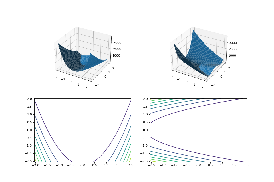
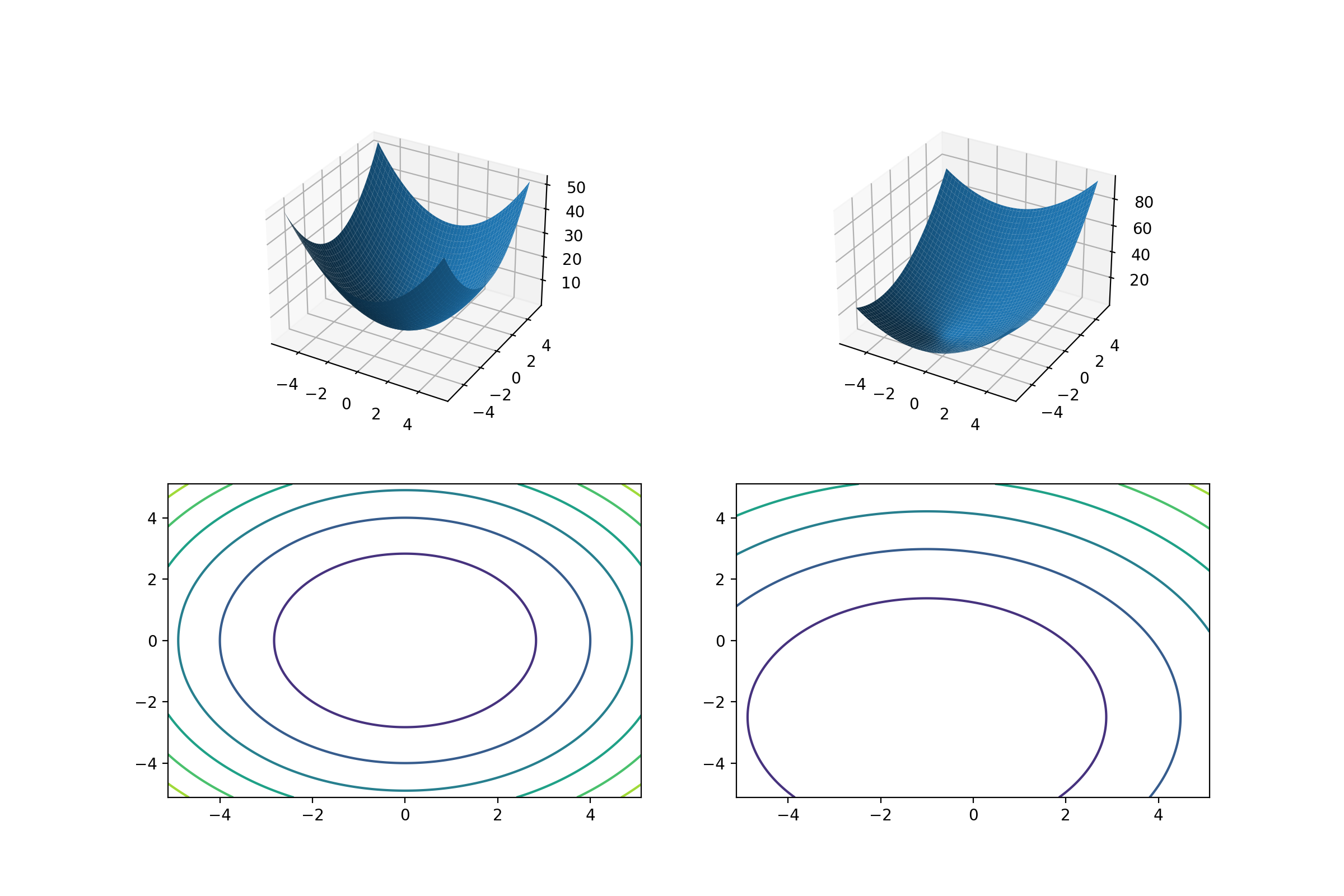
- class leap_ec.real_rep.problems.MatrixTransformedProblem(problem, matrix, maximize=None)
Bases:
ScalarProblemApply a linear transformation to a fitness function.
- Parameters
matrix – an nxn matrix, where n is the genome length.
- Returns
a function that first applies -matrix to the input, then applies fun to the transformed input.
For example, here we manually construct a 2x2 rotation matrix and apply it to the
leap.RosenbrockProblemfunction:from matplotlib import pyplot as plt from leap_ec.real_rep.problems import RosenbrockProblem, MatrixTransformedProblem, plot_2d_problem original_problem = RosenbrockProblem() theta = np.pi/2 matrix = [[np.cos(theta), -np.sin(theta)], [np.sin(theta), np.cos(theta)]] transformed_problem = MatrixTransformedProblem(original_problem, matrix) fig = plt.figure(figsize=(12, 8)) plt.subplot(221, projection='3d') bounds = RosenbrockProblem.bounds # Contains traditional bounds plot_2d_problem(original_problem, xlim=bounds, ylim=bounds, ax=plt.gca(), granularity=0.025) plt.subplot(222, projection='3d') plot_2d_problem(transformed_problem, xlim=bounds, ylim=bounds, ax=plt.gca(), granularity=0.025) plt.subplot(223) plot_2d_problem(original_problem, kind='contour', xlim=bounds, ylim=bounds, ax=plt.gca(), granularity=0.025) plt.subplot(224) plot_2d_problem(transformed_problem, kind='contour', xlim=bounds, ylim=bounds, ax=plt.gca(), granularity=0.025)
(Source code, png, hires.png, pdf)
- evaluate(phenome)
Evaluated the fitness of a point on the transformed fitness landscape.
For example, consider a sphere function whose global optimum is situated at (0, 1):
>>> import numpy as np
>>> s = TranslatedProblem(SpheroidProblem(), offset=[0, 1])
>>> np.round(s.evaluate(np.array([0, 1])), 5)
np.int64(0)
Now let’s take a rotation matrix that transforms the space by pi/2 radians:
>>> import numpy as np
>>> theta = np.pi/2
>>> matrix = [[np.cos(theta), -np.sin(theta)],                      [np.sin(theta), np.cos(theta)]]
>>> r = MatrixTransformedProblem(s, matrix)
The rotation has moved the new global optimum to (1, 0)
>>> np.round(r.evaluate(np.array([1, 0])), 5)
np.float64(0.0)
The point (0, 1) lies at a distance of sqrt(2) from the new optimum, and has a fitness of 2:
>>> np.round(r.evaluate(np.array([0, 1])), 5)
np.float64(2.0)
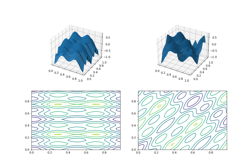
- classmethod random_orthonormal(problem, dimensions, maximize=None)
Create a
MatrixTransformedProblemthat performs a random rotation and/or inversion of the function.We accomplish this by generating a random orthonormal basis for R^n and plugging the resulting matrix into
MatrixTransformedProblem.The classic algorithm we use here is based on the Gramm-Schmidt process: we first generate a set of random vectors, and then convert them into an orthonormal basis. This approach is described in Hansen and Ostermeier’s original CMA-ES paper:
“Completely derandomized self-adaptation in evolution strategies.” Evolutionary Computation 9.2 (2001): 159-195.
- Parameters
problem – the original
ScalarProblemto apply the transform to.dimensions (int) – the number of elements each vector should have.
maximize (bool) – whether to maximize or minimize the resulting fitness function. Defaults to whatever setting the underlying problem uses.
from matplotlib import pyplot as plt
from leap_ec.real_rep.problems import CosineFamilyProblem, MatrixTransformedProblem, plot_2d_problem

original_problem = CosineFamilyProblem(alpha=1.0, global_optima_counts=[2, 3], local_optima_counts=[2, 3])

transformed_problem = MatrixTransformedProblem.random_orthonormal(original_problem, 2)

fig = plt.figure(figsize=(12, 8))

plt.subplot(221, projection='3d')
bounds = original_problem.bounds
plot_2d_problem(original_problem, xlim=bounds, ylim=bounds, ax=plt.gca(), granularity=0.025)

plt.subplot(222, projection='3d')
plot_2d_problem(transformed_problem, xlim=bounds, ylim=bounds, ax=plt.gca(), granularity=0.025)

plt.subplot(223)
plot_2d_problem(original_problem, kind='contour', xlim=bounds, ylim=bounds, ax=plt.gca(), granularity=0.025)

plt.subplot(224)
plot_2d_problem(transformed_problem, kind='contour', xlim=bounds, ylim=bounds, ax=plt.gca(), granularity=0.025)
(Source code, png, hires.png, pdf)
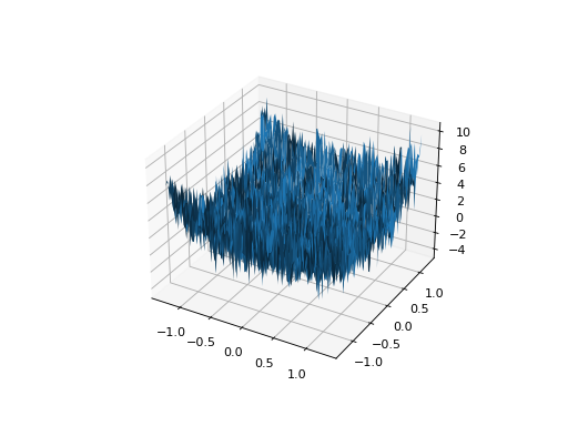
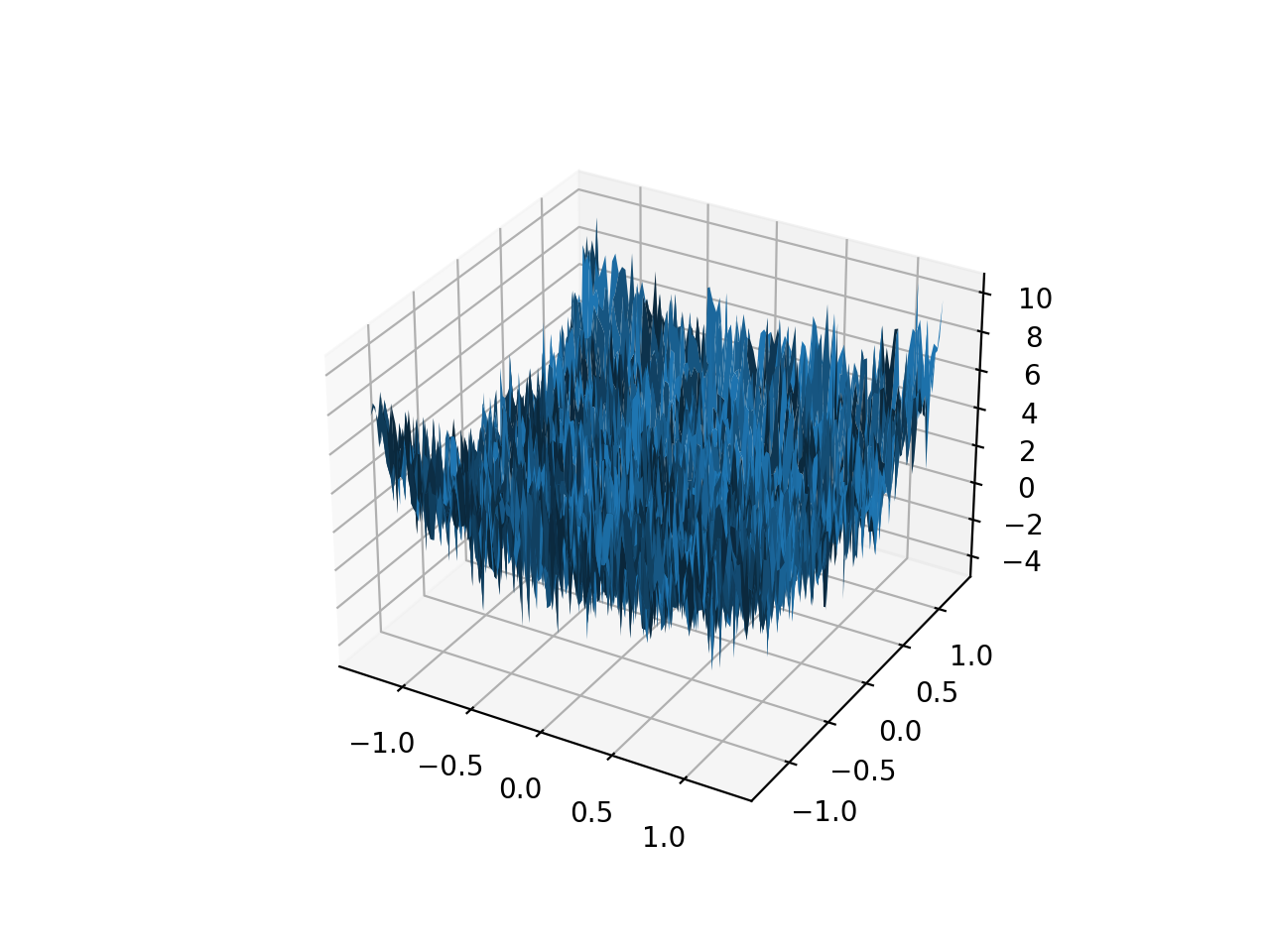
- class leap_ec.real_rep.problems.NoisyQuarticProblem(maximize=False)
Bases:
ScalarProblemThe classic ‘quadratic quartic’ function with Gaussian noise:
\[f(\mathbf{x}) = \sum_{i=1}^{n} i x_i^4 + \texttt{gauss}(0, 1)\]- Parameters
maximize (bool) – the function is maximized if True, else minimized.
from leap_ec.real_rep.problems import NoisyQuarticProblem, plot_2d_problem
bounds = NoisyQuarticProblem.bounds  # Contains traditional bounds
plot_2d_problem(NoisyQuarticProblem(), xlim=bounds, ylim=bounds, granularity=0.025)
(Source code, png, hires.png, pdf)

- bounds = (-1.28, 1.28)
- evaluate(phenome)
Computes the function value from a real-valued list phenome (the output varies, since the function has noise):
>>> phenome = [3.5, -3.8, 5.0]
>>> r = NoisyQuarticProblem().evaluate(phenome)
>>> print(f'Result: {r}')
Result: ...
- Parameters
phenome – real-valued vector to be evaluated
- Returns
its fitness
- worse_than(first_fitness, second_fitness)
We minimize by default:
>>> s = NoisyQuarticProblem()
>>> s.worse_than(100, 10)
True
>>> s = NoisyQuarticProblem(maximize=True)
>>> s.worse_than(100, 10)
False
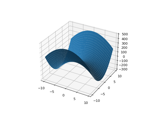
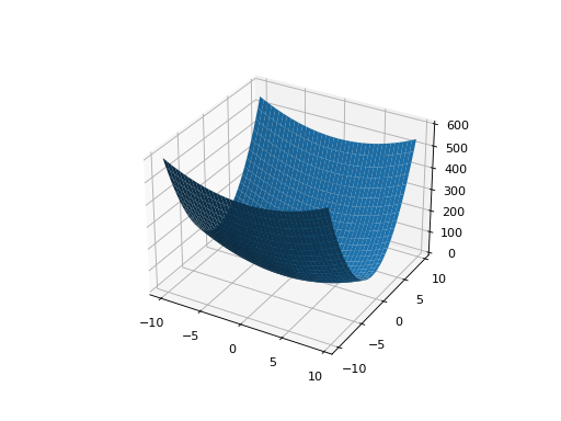
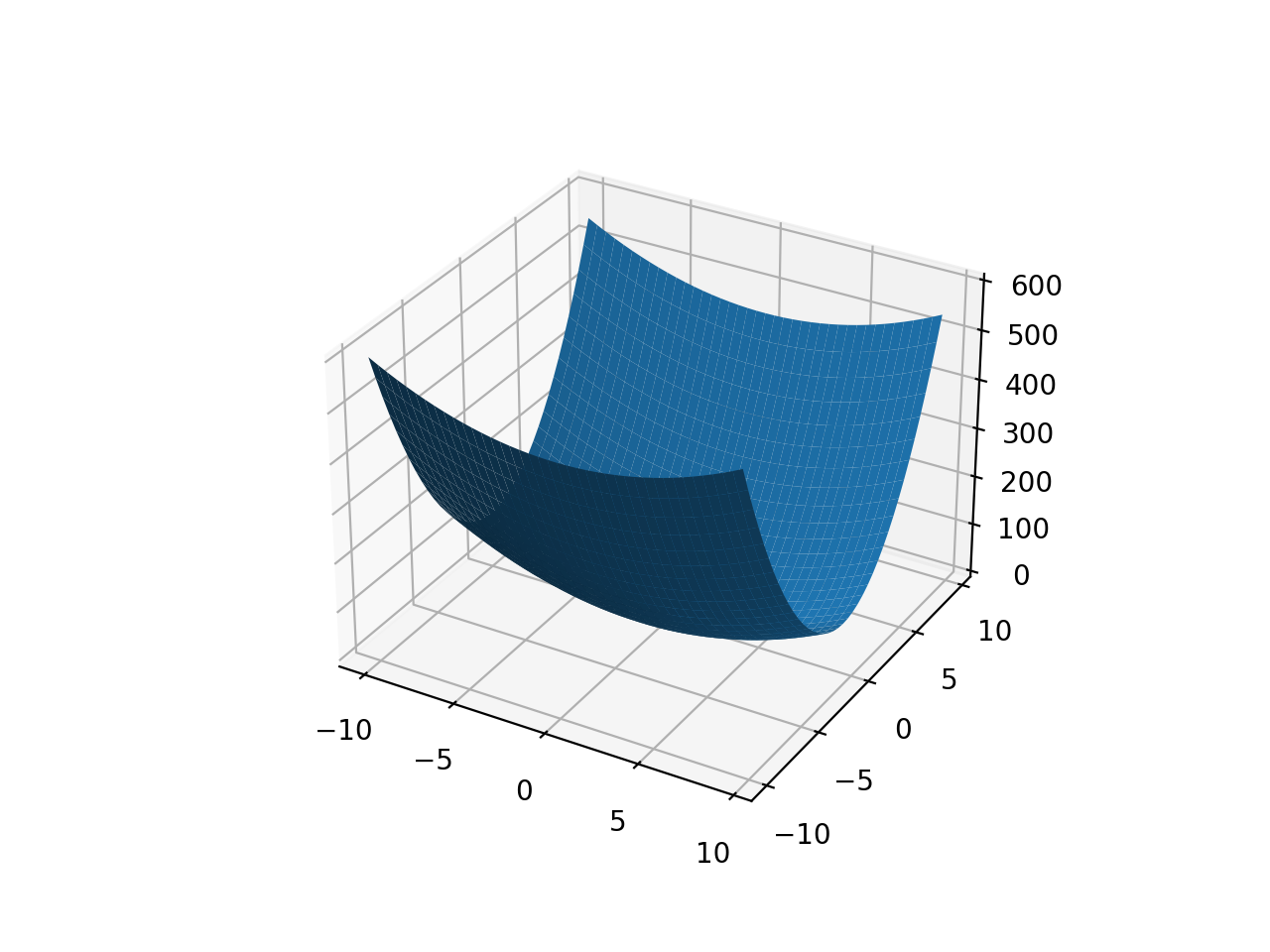
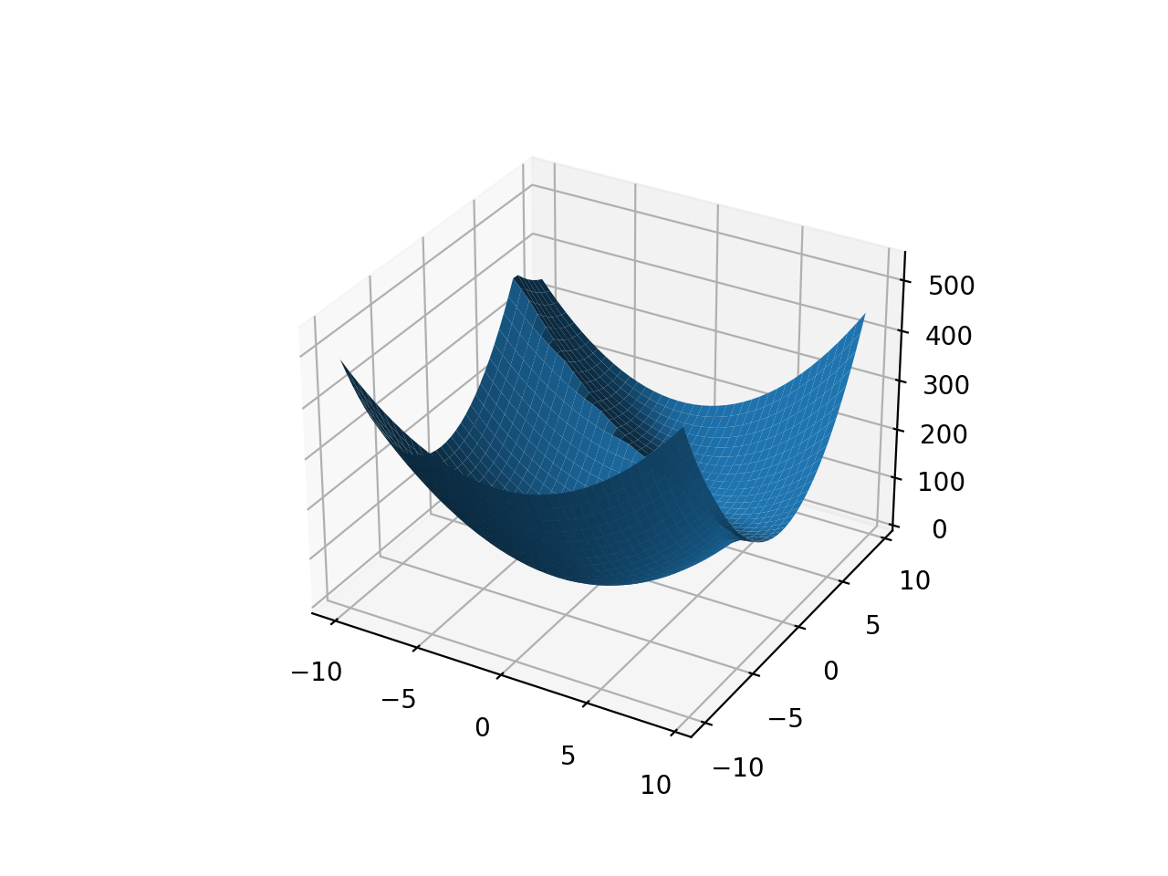
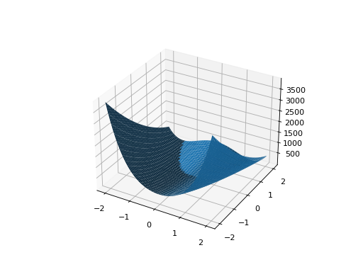
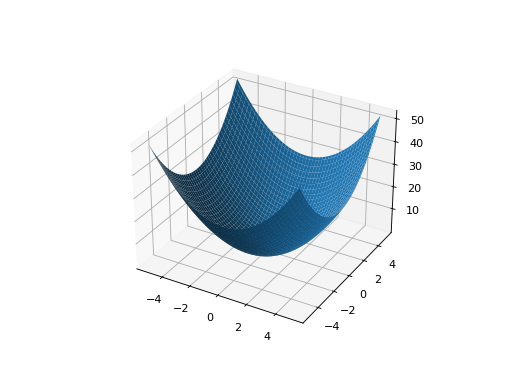
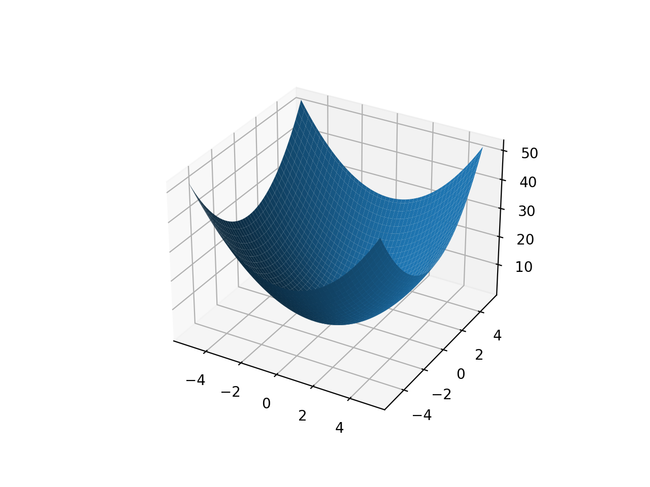
- class leap_ec.real_rep.problems.ParabaloidProblem(diagonal_matrix: ndarray, rotation_matrix: ndarray, maximize=False)
Bases:
ScalarProblemA generalization of the SpheroidProblem into parabaloids (including elliptic and hyperbolic parabaloids).
We construct the parabaloid by combining a diagonal matrix (which defines an axis-aligned parabaloid) with an orthornormal rotation. Together, these make up the eigenvalues and eigenbasis, respectively, of an arbitrary parabaloid:
\[\mathbf{A} = \mathbf{R}^\top \mathbf{D} \mathbf{R}\]We then compute fitness by interpretting \(A\) as a quadratic form:
\[f(x) = x^\top \mathbf{A} x\]When the eigenvalues are all positive, then the result is an elliptic parabaloid
from leap_ec.real_rep .problems import ParabaloidProblem, plot_2d_problem
from matplotlib import pyplot as plt
import numpy as np

p = ParabaloidProblem(diagonal_matrix=np.diag([1, 5]), rotation_matrix=np.identity(2))
plot_2d_problem(p, xlim=(-10, 10), ylim=(-10, 10), granularity=0.5)
plt.show()
(Source code, png, hires.png, pdf)

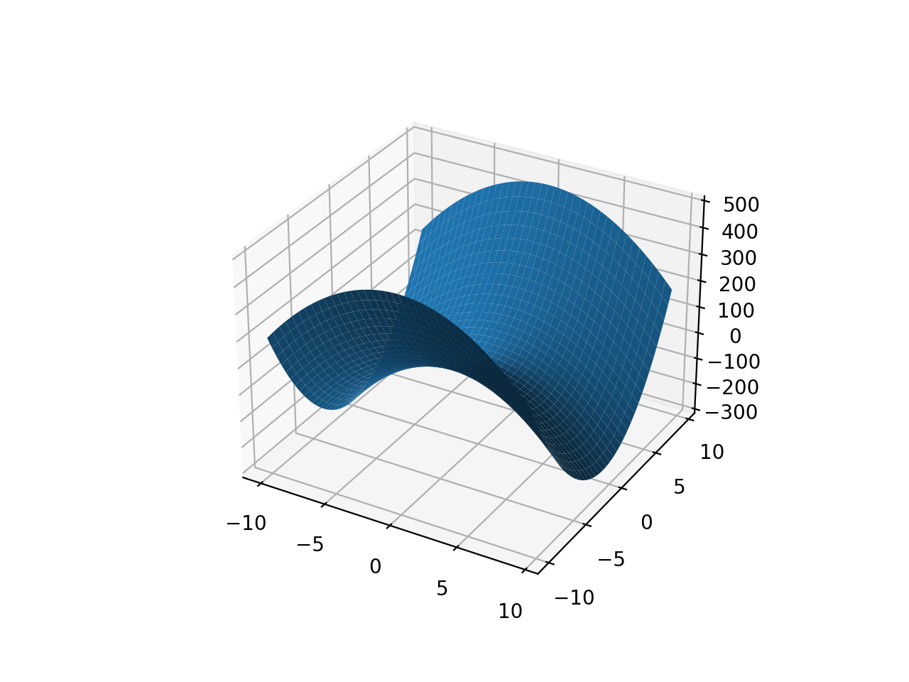
If one or more eigenvalues are negative, then a hyperbolic parabloid results, which has a saddle shape:
from leap_ec.real_rep .problems import ParabaloidProblem, plot_2d_problem
from matplotlib import pyplot as plt
import numpy as np

p = ParabaloidProblem(diagonal_matrix=np.diag([-3, 5]), rotation_matrix=np.identity(2))
plot_2d_problem(p, xlim=(-10, 10), ylim=(-10, 10), granularity=0.5)
plt.show()
(Source code, png, hires.png, pdf)
- evaluate(phenome)
Evaluate the given phenome.
Practitioners must over-ride this member function.
Note that by default the individual comparison operators assume a maximization problem; if this is a minimization problem, then just negate the value when returning the fitness.
- Parameters
phenome – the phenome to evaluate (this will not be modified)
- Returns
the fitness value
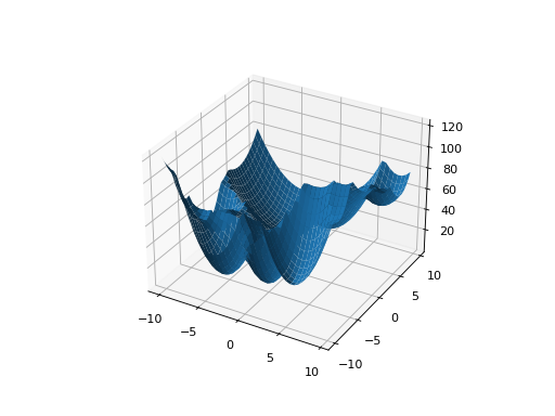
- class leap_ec.real_rep.problems.QuadraticFamilyProblem(diagonal_matrices: list, rotation_matrices: list, offset_vectors: list, fitness_offsets: list, maximize=False)
Bases:
ScalarProblemA configurable multi-modal function based on combinations of spheroids or parabaloids. Taken from the problem generators proposed by Rönkkönen et al. [RonkkonenLKL08].
The function is given by
\[f(\mathbf{x}) = \min_{i=1,2,\dots,q} \left( (\mathbf{x} - \mathbf{p}_i)^\top \mathbf{B}_i^{-1} (\mathbf{x} - \mathbf{p}_i) + v_i \right)\]where the \(\mathbf{p}_i\) gives the center of each quadratic (i.e. the location of each local minimum), the \(v_i\) give their fitness values, and the \(\mathbf{B}_i^{-1}\) are symmetric matrices.
The easiest way to create one of these problems is to use the random generator:
from leap_ec.real_rep.problems import QuadraticFamilyProblem, plot_2d_problem
from matplotlib import pyplot as plt

problem = QuadraticFamilyProblem.generate(dimensions=2, num_basins=30)
plot_2d_problem(problem, xlim=(-10, 10), ylim=(-10, 10), granularity=0.5)
plt.show()
(Source code, png, hires.png, pdf)
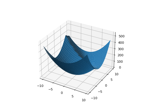
You can also specify the problem structure directly by providing two matrices for each parabaloid along with an offset vector (for translation) and a scalar offset (to define the minimum fitness value for the basin):
from leap_ec.real_rep.problems import QuadraticFamilyProblem, plot_2d_problem, random_orthonormal_matrix
from matplotlib import pyplot as plt
import numpy as np

# Define the parameters for each parabaloid

diag1 = np.diag([2, 4])     # Diagonal matrix defining the widths (eigenvalues) of the basin for each dimension
rot1 = np.identity(2)       # Rotation matrix, in this case the identity (no rotation)
offset1 = np.array([-1, -1])  # Offset used to translate the basin location
fitness1 = 0                # Fitness value of the local optimum

diag2 = np.diag([5, 1])
rot2 = random_orthonormal_matrix(dimensions=2)  # Apply a random rotation to the second basin
offset2 = np.array([3, 4])
fitness2 = 100.0

# Build the problem
problem = QuadraticFamilyProblem(
    diagonal_matrices = [ diag1, diag2 ],
    rotation_matrices = [ rot1, rot2 ],
    offset_vectors = [ offset1, offset2 ],
    fitness_offsets = [ fitness1, fitness2 ]
)

# Visualize
plot_2d_problem(problem, xlim=(-10, 10), ylim=(-10, 10), granularity=0.5)
plt.show()
(Source code, png, hires.png, pdf)
- property dimensions
- evaluate(phenome)
Evaluate the given phenome.
Practitioners must over-ride this member function.
Note that by default the individual comparison operators assume a maximization problem; if this is a minimization problem, then just negate the value when returning the fitness.
- Parameters
phenome – the phenome to evaluate (this will not be modified)
- Returns
the fitness value
- classmethod generate(dimensions: int, num_basins: int, num_global_optima: int = 1, width_bounds: tuple = (1, 5), offset_bounds: tuple = (-10, 10), fitness_offset_bounds: tuple = (10, 100))
Convenient method to generate a QuadraticFamilyProblem by randomly sampling the matrices that define it.
>>> problem = QuadraticFamilyProblem.generate(10, 20, num_global_optima = 2)
>>> x = problem.evaluate(np.array([0.0, 0.5, 0.0, 0.6, 0.0, 0.7, 0.6, 0.8, 4.3, 0.2]))
- property num_basins
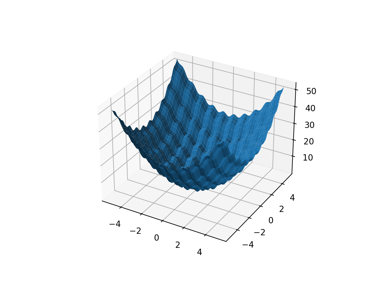
- class leap_ec.real_rep.problems.RastriginProblem(a=1.0, maximize=False)
Bases:
ScalarProblemThe classic Rastrigin problem. The Rastrigin provides a real-valued fitness landscape with a quadratic global structure (like the
SpheroidProblem), plus a sinusoidal local structure with many local optima.\[f(\vec{x}) = An + \sum_{i=1}^n x_i^2 - A\cos(2\pi x_i)\]- Parameters
maximize (bool) – the function is maximized if True, else minimized.
from leap_ec.real_rep.problems import RastriginProblem, plot_2d_problem
bounds = RastriginProblem.bounds  # Contains traditional bounds
plot_2d_problem(RastriginProblem(), xlim=bounds, ylim=bounds, granularity=0.025)
(Source code, png, hires.png, pdf)
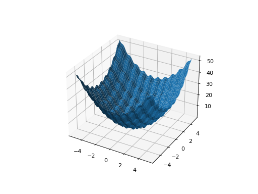
- bounds = (-5.12, 5.12)
- evaluate(phenome)
Computes the function value from a real-valued list phenome:
>>> phenome = [1.0/12, 0]
>>> RastriginProblem().evaluate(phenome)
np.float64(0.1409190406...)
- Parameters
phenome – real-valued vector to be evaluated
- Returns
its fitness
- worse_than(first_fitness, second_fitness)
We minimize by default:
>>> s = RastriginProblem()
>>> s.worse_than(100, 10)
True
>>> s = RastriginProblem(maximize=True)
>>> s.worse_than(100, 10)
False
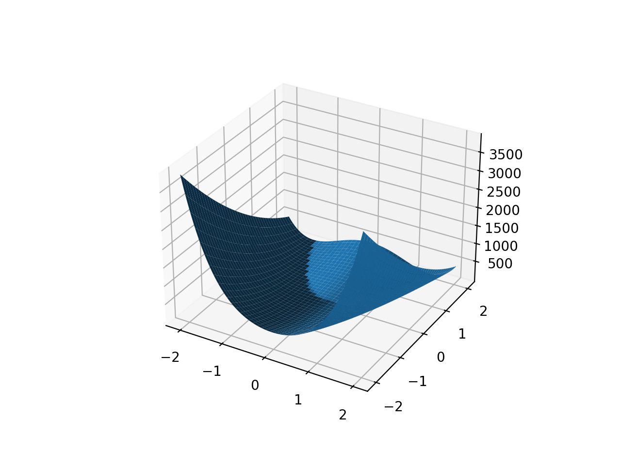
- class leap_ec.real_rep.problems.RosenbrockProblem(maximize=False)
Bases:
ScalarProblemThe classic RosenbrockProblem problem, a.k.a. the “banana” or “valley” function.
\[f(\mathbf{x}) = \sum_{i=1}^{d-1} \left[ 100 (x_{i + 1} - x_i^2)^2 + (x_i - 1)^2\right]\]- Parameters
maximize (bool) – the function is maximized if True, else minimized.
from leap_ec.real_rep.problems import RosenbrockProblem, plot_2d_problem
bounds = RosenbrockProblem.bounds  # Contains traditional bounds
plot_2d_problem(RosenbrockProblem(), xlim=bounds, ylim=bounds, granularity=0.025)
(Source code, png, hires.png, pdf)

- bounds = (-2.048, 2.048)
- evaluate(phenome)
Computes the function value from a real-valued list phenome:
>>> phenome = [0.5, -0.2, 0.1]
>>> RosenbrockProblem().evaluate(phenome)
22.3
- Parameters
phenome – real-valued vector to be evaluated
- Returns
its fitness
- worse_than(first_fitness, second_fitness)
We minimize by default:
>>> s = RosenbrockProblem()
>>> s.worse_than(100, 10)
True
>>> s = RosenbrockProblem(maximize=True)
>>> s.worse_than(100, 10)
False
- class leap_ec.real_rep.problems.ScaledProblem(problem, new_bounds, maximize=None)
Bases:
ScalarProblemScale the search space of a fitness function up or down.
- evaluate(phenome)
Evaluate the given phenome.
Practitioners must over-ride this member function.
Note that by default the individual comparison operators assume a maximization problem; if this is a minimization problem, then just negate the value when returning the fitness.
- Parameters
phenome – the phenome to evaluate (this will not be modified)
- Returns
the fitness value
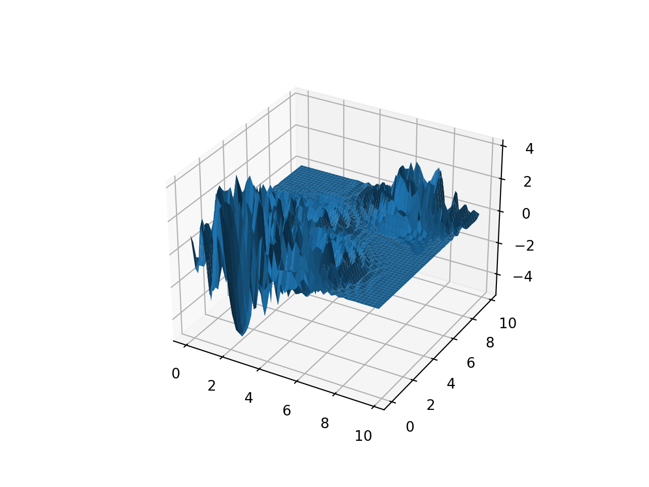
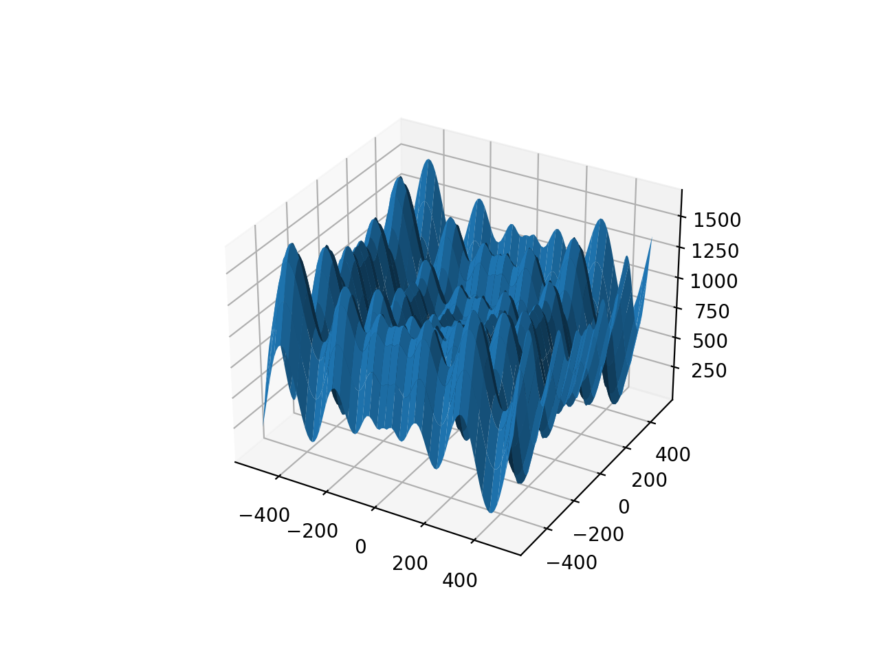
- class leap_ec.real_rep.problems.SchwefelProblem(alpha=418.982887, maximize=False)
Bases:
ScalarProblemSchwefel’s function is another traditional multimodal test function whose local optima are distributed in a slightly irregular way, and whose global optimum is out at the edge of the search space (with no gently sloping macrostructure to guide the algorithm toward it).
Compare this to the
RastriginProblemfunction, whose global optimum lies at the center of a quadratic bowl with a regular grid of local optima.\[f(\mathbf{x}) = \sum_{i=1}^d\left(-x_i \cdot\sin\left(\sqrt{|x_i|} \right)\right) + \alpha \cdot d\]- Parameters
alpha (float) – fitness offset (the default value ensures that the global optimum has zero fitness)
maximize (bool) – the function is maximized if True, else minimized.
from leap_ec.real_rep.problems import SchwefelProblem, plot_2d_problem
bounds = SchwefelProblem.bounds  # Contains traditional bounds
plot_2d_problem(SchwefelProblem(), xlim=bounds, ylim=bounds, granularity=10)
(Source code, png, hires.png, pdf)

- bounds = (-512, 512)
- evaluate(phenome)
Computes the function value from a real-valued phenome.
- Parameters
phenome – phenome with a real-valued phenome to be evaluated
- Returns
its fitness.
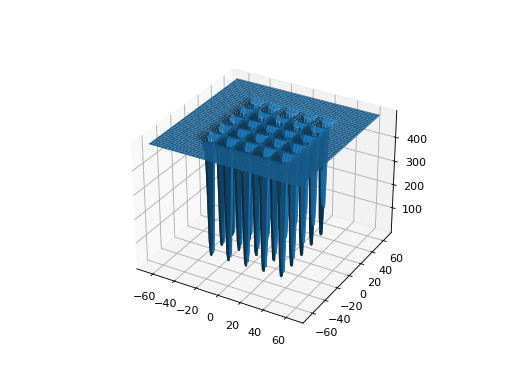
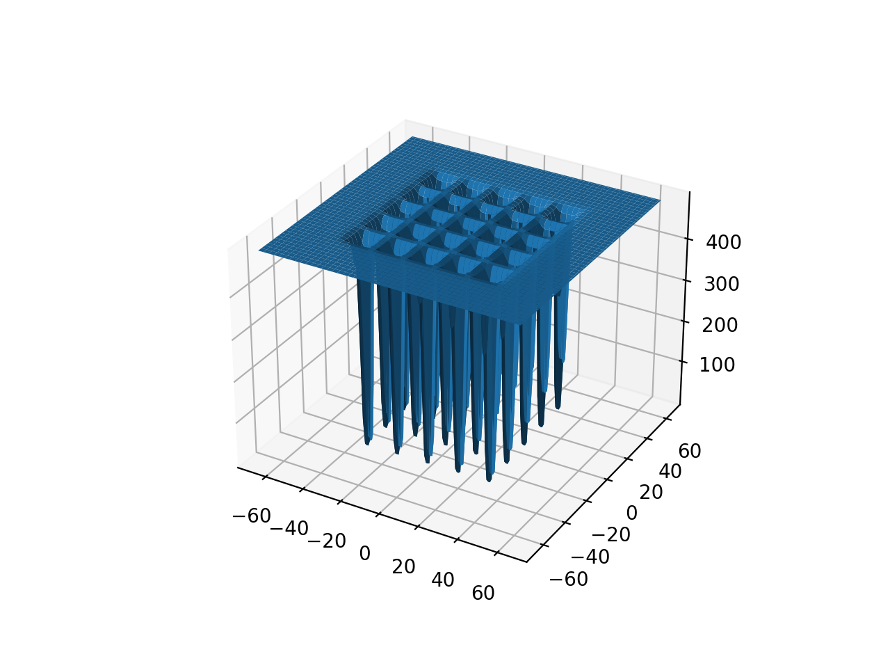
- class leap_ec.real_rep.problems.ShekelProblem(k=500, c=array([1, 2, 3, 4, 5, 6, 7, 8, 9, 10, 11, 12, 13, 14, 15, 16, 17, 18, 19, 20, 21, 22, 23, 24, 25]), maximize=False)
Bases:
ScalarProblemThe classic ‘Shekel’s foxholes’ function.
\[f(\mathbf{x}) = \frac{1}{\frac{1}{K} + \sum_{j=1}^{25} \frac{1}{f_j(\mathbf{x})}}\]where
\[f_j(\mathbf{x}) = c_j + \sum_{i=1}^2 (x_i - a_{ij})^6\]and the points \(\left\{ (a_{1j}, a_{2j})\right\}_{j=1}^{25}\) define the functions various optima, and are given by the following hardcoded matrix:
\[\begin{split}\left[a_{ij}\right] = \left[ \begin{array}{lllllllllll} -32 & -16 & 0 & 16 & 32 & -32 & -16 & \cdots & 0 & 16 & 32 \\ -32 & -32 & -32 & -32 & -32 & -16 & -16 & \cdots & 32 & 32 & 32 \end{array} \right].\end{split}\]- Parameters
k (int) – the value of \(K\) in the fitness function.
c ([int]) – list of values for the function’s \(c_j\) parameters. Each c[j] approximately corresponds to the depth of the jth foxhole.
maximize (bool) – the function is maximized if True, else minimized.
maximize – the function is maximized if True, else minimized.
from leap_ec.real_rep.problems import ShekelProblem, plot_2d_problem
bounds = ShekelProblem.bounds  # Contains traditional bounds
plot_2d_problem(ShekelProblem(), xlim=bounds, ylim=bounds, granularity=0.9)
(Source code, png, hires.png, pdf)

- bounds = (-65.536, 65.536)
- evaluate(phenome)
Computes the function value from a real-valued list phenome (the output varies, since the function has noise).
- Parameters
phenome – real-valued to be evaluated
- Returns
its fitness
- points = array([[-32, -16, 0, 16, 32, -32, -16, 0, 16, 32, -32, -16, 0, 16, 32, -32, -16, 0, 16, 32, -32, -16, 0, 16, 32], [-32, -32, -32, -32, -32, -16, -16, -16, -16, -16, 0, 0, 0, 0, 0, 16, 16, 16, 16, 16, 32, 32, 32, 32, 32]])
- worse_than(first_fitness, second_fitness)
We minimize by default:
>>> s = ShekelProblem()
>>> s.worse_than(100, 10)
True
>>> s = ShekelProblem(maximize=True)
>>> s.worse_than(100, 10)
False
- class leap_ec.real_rep.problems.SpheroidProblem(maximize=False)
Bases:
ScalarProblemClassic paraboloid function, known as the “sphere” or “spheroid” problem, because its equal-fitness contours form (hyper)spheres in n > 2.
\[f(\vec{x}) = \sum_{i}^n x_i^2\]- Parameters
maximize (bool) – the function is maximized if True, else minimized.
from leap_ec.real_rep.problems import SpheroidProblem, plot_2d_problem
bounds = SpheroidProblem.bounds  # Contains traditional bounds
plot_2d_problem(SpheroidProblem(), xlim=bounds, ylim=bounds, granularity=0.025)
(Source code, png, hires.png, pdf)
- bounds = (-5.12, 5.12)
- evaluate(phenome)
Computes the function value from a real-valued list phenome:
>>> phenome = [0.5, 0.8, 1.5]
>>> SpheroidProblem().evaluate(phenome)
3.14
- Parameters
phenome – real-valued vector to be evaluated
- Returns
it’s fitness, sum(phenome**2)
- worse_than(first_fitness, second_fitness)
We minimize by default:
>>> s = SpheroidProblem()
>>> s.worse_than(100, 10)
True
>>> s = SpheroidProblem(maximize=True)
>>> s.worse_than(100, 10)
False
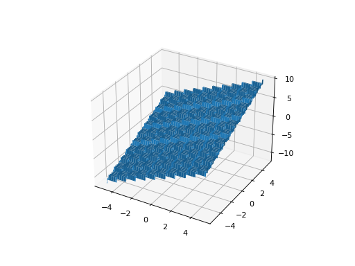
- class leap_ec.real_rep.problems.StepProblem(maximize=True)
Bases:
ScalarProblemThe classic ‘step’ function—a function with a linear global structure, but with stair-like plateaus at the local level.
\[f(\mathbf{x}) = \sum_{i=1}^{n} \lfloor x_i \rfloor\]where \(\lfloor x \rfloor\) denotes the floor function.
- Parameters
maximize (bool) – the function is maximized if True, else minimized.
from leap_ec.real_rep.problems import StepProblem, plot_2d_problem
bounds = StepProblem.bounds  # Contains traditional bounds
plot_2d_problem(StepProblem(), xlim=bounds, ylim=bounds, granularity=0.025)
(Source code, png, hires.png, pdf)
- bounds = (-5.12, 5.12)
- evaluate(phenome)
Computes the function value from a real-valued list phenome:
>>> import numpy as np
>>> phenome = np.array([3.5, -3.8, 5.0])
>>> StepProblem().evaluate(phenome)
np.float64(4.0)
- Parameters
phenome – real-valued vector to be evaluated
- Returns
its fitness
- worse_than(first_fitness, second_fitness)
We maximize by default:
>>> s = StepProblem()
>>> s.worse_than(100, 10)
False
>>> s = StepProblem(maximize=False)
>>> s.worse_than(100, 10)
True
- class leap_ec.real_rep.problems.TranslatedProblem(problem, offset, maximize=None)
Bases:
ScalarProblemTakes an existing fitness function and translates it by applying a fixed offset vector.
For example,
from matplotlib import pyplot as plt
from leap_ec.real_rep.problems import SpheroidProblem, TranslatedProblem, plot_2d_problem

original_problem = SpheroidProblem()
offset = [-1.0, -2.5]
translated_problem = TranslatedProblem(original_problem, offset)

fig = plt.figure(figsize=(12, 8))

plt.subplot(221, projection='3d')
bounds = SpheroidProblem.bounds  # Contains traditional bounds
plot_2d_problem(original_problem, xlim=bounds, ylim=bounds, ax=plt.gca(), granularity=0.025)

plt.subplot(222, projection='3d')
plot_2d_problem(translated_problem, xlim=bounds, ylim=bounds, ax=plt.gca(), granularity=0.025)

plt.subplot(223)
plot_2d_problem(original_problem, kind='contour', xlim=bounds, ylim=bounds, ax=plt.gca(), granularity=0.025)

plt.subplot(224)
plot_2d_problem(translated_problem, kind='contour', xlim=bounds, ylim=bounds, ax=plt.gca(), granularity=0.025)
(Source code, png, hires.png, pdf)

- evaluate(phenome)
Evaluate the fitness of a point after translating the fitness function.
Translation can be used in higher than two dimensions:
>>> import numpy as np
>>> offset = [-1.0, -1.0, 1.0, 1.0, -5.0]
>>> t_sphere = TranslatedProblem(SpheroidProblem(), offset)
>>> genome = np.array([0.5, 2.0, 3.0, 8.5, -0.6])
>>> t_sphere.evaluate(genome)
np.float64(90.86)
- classmethod random(problem, offset_bounds, dimensions, maximize=None)
Apply a random real-valued translation to a fitness function, sampled uniformly between min_offset and max_offset in every dimension.
>>> from leap_ec.real_rep.problems import TranslatedProblem, RastriginProblem, plot_2d_problem
>>> original_problem = RastriginProblem()
>>> bounds = RastriginProblem.bounds  # Contains traditional bounds
>>> translated_problem = TranslatedProblem.random(original_problem, bounds, 2)
>>> plot_2d_problem(translated_problem, kind='contour', xlim=bounds, ylim=bounds)
<matplotlib.contour...>
from leap_ec.real_rep.problems import TranslatedProblem, RastriginProblem, plot_2d_problem

original_problem = RastriginProblem()
bounds = RastriginProblem.bounds  # Contains traditional bounds
translated_problem = TranslatedProblem.random(original_problem, bounds, 2)

plot_2d_problem(translated_problem, kind='contour', xlim=bounds, ylim=bounds)
(Source code, png, hires.png, pdf)

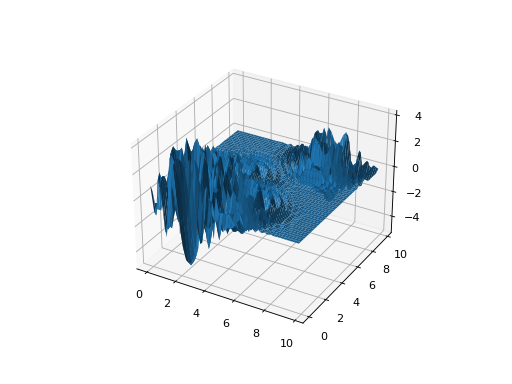
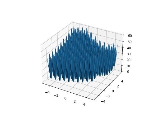
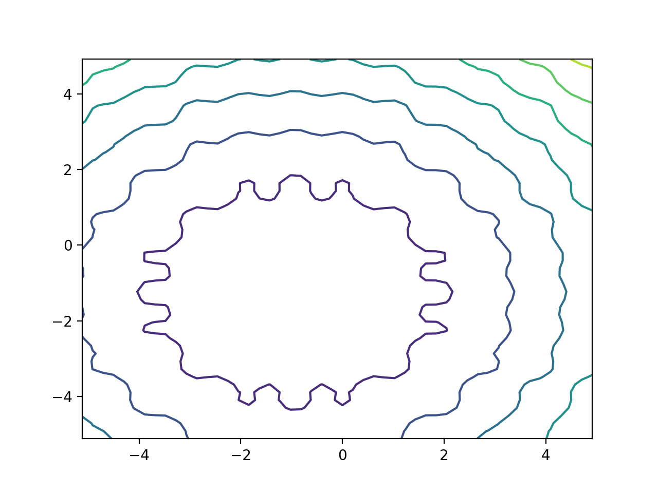
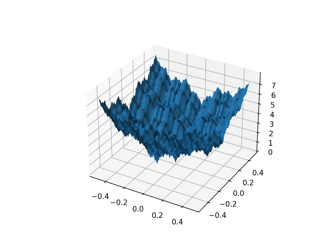
- class leap_ec.real_rep.problems.WeierstrassProblem(kmax=20, a=0.5, b=3, maximize=False)
Bases:
ScalarProblemThe Weierstrass function is famous for being the first discovered example of a function that is continuous, but not differentiable. Built by adding the terms of a Fourier series, it has a jagged, self-similar structure:
\[f(\mathbf{x}) = \sum_{i=1}^d \left[ \sum_{k=0}^{kmax} a^k \cos\left( 2\pi b^k(x_i + 0.5)\right) - n \sum_{k=0}^{kmax} a^k \cos(\pi b^k) \right]\]When used in optimization benchmarks, it’s typical to carry out the Fourier sum to kmax=20 terms.
- Parameters
kmax (int) – number of terms to carry the Fourier sum out to
a (float) – amplitude parameter of the cosine terms
b (float) – wavenumber (frequency) parameter of the cosine terms
maximize (bool) – the function is maximized if True, else minimized.
from leap_ec.real_rep.problems import WeierstrassProblem, plot_2d_problem
bounds = WeierstrassProblem.bounds  # Contains traditional bounds
plot_2d_problem(WeierstrassProblem(), xlim=bounds, ylim=bounds, granularity=0.01)
(Source code, png, hires.png, pdf)

- bounds = [-0.5, 0.5]
- evaluate(phenome)
Computes the function value from a real-valued phenome.
- Parameters
phenome – real-valued vector to be evaluated
- Returns
its fitness.
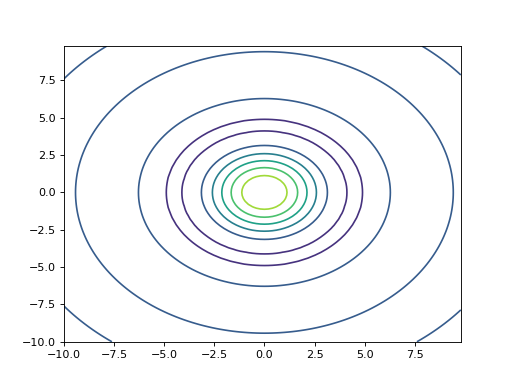
- leap_ec.real_rep.problems.plot_2d_contour(fun, xlim, ylim, granularity, ax=None, title=None, pad=None)
Convenience method for plotting contours for a function that accepts 2-D real-valued inputs and produces a 1-D scalar output.
- Parameters
fun (function) – The function to plot.
xlim ((float, float)) – Bounds of the horizontal axes.
ylim ((float, float)) – Bounds of the vertical axis.
ax (Axes) – Matplotlib axes to plot to (if None, a new figure will be created).
granularity (float) – Spacing of the grid to sample points along.
pad – An array of extra gene values, used to fill in the hidden dimensions with contants while drawing fitness contours.
The difference between this and
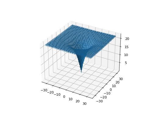
plot_2d_problem()is that this takes a raw function (instead of aProblemobject).import numpy as np from scipy import linalg from leap_ec.real_rep.problems import plot_2d_contour def sinc_hd(phenome): r = linalg.norm(phenome) return np.sin(r)/r plot_2d_contour(sinc_hd, xlim=(-10, 10), ylim=(-10, 10), granularity=0.2)
(Source code, png, hires.png, pdf)

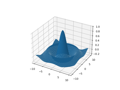
- leap_ec.real_rep.problems.plot_2d_function(fun, xlim, ylim, granularity=0.1, ax=None, title=None, pad=None, **kwargs)
Convenience method for plotting a function that accepts 2-D real-valued imputs and produces a 1-D scalar output.
- Parameters
fun (function) – The function to plot.
xlim ((float, float)) – Bounds of the horizontal axes.
ylim ((float, float)) – Bounds of the vertical axis.
ax (Axes) – Matplotlib axes to plot to (if None, a new figure will be created).
granularity (float) – Spacing of the grid to sample points along.
pad – An array of extra gene values, used to fill in the hidden dimensions with contants while drawing fitness contours.
kwargs – additional keyword arguments to pass along to plot_surface() or contour()
The difference between this and
plot_2d_problem()is that this takes a raw function (instead of aProblemobject).import numpy as np from scipy import linalg from leap_ec.real_rep.problems import plot_2d_function def sinc_hd(phenome): r = linalg.norm(phenome) return np.sin(r)/r plot_2d_function(sinc_hd, xlim=(-10, 10), ylim=(-10, 10), granularity=0.2)
(Source code, png, hires.png, pdf)

- leap_ec.real_rep.problems.plot_2d_problem(problem, xlim=None, ylim=None, kind='surface', ax=None, granularity=None, title=None, pad=None, **kwargs)
Convenience function for plotting a
Problemthat accepts 2-D real-valued phenomes and produces a 1-D scalar fitness output.- Parameters
fun (Problem) – The
Problemto plot.xlim ((float, float)) – Bounds of the horizontal axes. If None, uses problem.bounds.
ylim ((float, float)) – Bounds of the vertical axis. If None, uses problem.bounds.
kind (str) – The kind of plot to create: ‘surface’ or ‘contour’
pad – An array of extra gene values, used to fill in the hidden dimensions with contants while drawing fitness contours.
ax (Axes) – Matplotlib axes to plot to (if None, a new figure will be created).
granularity (float) – Spacing of the grid to sample points along. If none is given, then the granularity will default to 1/50th of the range of the function’s bounds attribute.
kwargs – additional keyword arguments to pass along to plot_surface()
The difference between this and
plot_2d_function()is that this takes aProblemobject (instead of a raw function).If no axes are specified, a new figure is created for the plot:
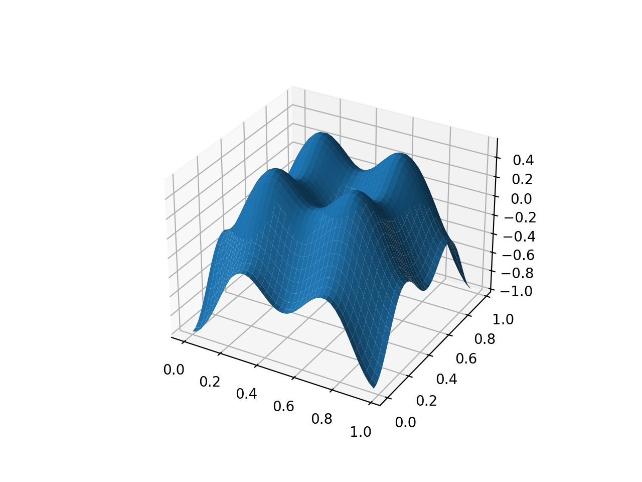
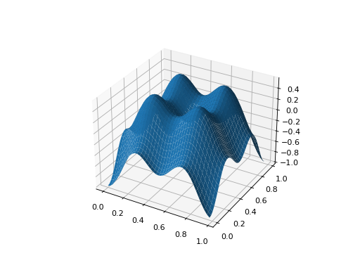
from leap_ec.real_rep.problems import CosineFamilyProblem, plot_2d_problem
problem = CosineFamilyProblem(alpha=1.0, global_optima_counts=[2, 2], local_optima_counts=[2, 2])
plot_2d_problem(problem, xlim=(0, 1), ylim=(0, 1), granularity=0.025);
(Source code, png, hires.png, pdf)

You can also specify axes explicitly (ex. by using ax=plt.gca(). When plotting surfaces, you must configure your axes to use projection=’3d’. Contour plots don’t need 3D axes:
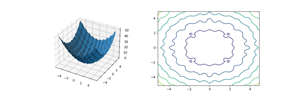
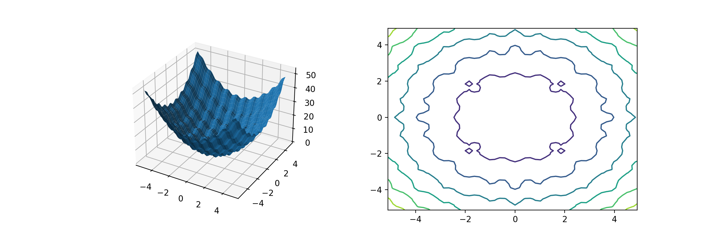
from matplotlib import pyplot as plt
from leap_ec.real_rep.problems import RastriginProblem, plot_2d_problem

fig = plt.figure(figsize=(12, 4))
bounds=RastriginProblem.bounds  # Contains default bounds

plt.subplot(121, projection='3d')
plot_2d_problem(RastriginProblem(), ax=plt.gca(), xlim=bounds, ylim=bounds)

plt.subplot(122)
plot_2d_problem(RastriginProblem(), ax=plt.gca(), kind='contour', xlim=bounds, ylim=bounds)
(Source code, png, hires.png, pdf)
- leap_ec.real_rep.problems.random(size=None)
Return random floats in the half-open interval [0.0, 1.0). Alias for random_sample to ease forward-porting to the new random API.
- leap_ec.real_rep.problems.random_orthonormal_matrix(dimensions: int)
Generate a random orthornomal matrix using the Gramm-Schmidt process.
Orthonormal matrices represent rotations (and flips) of a space.
The defining property of an orthonormal matrix is that its transpose is its inverse:
>>> Q = random_orthonormal_matrix(10)
>>> np.allclose( Q.dot(Q.T), np.identity(10) )
True