leap_ec.landscape_features package
Submodules
leap_ec.landscape_features.exploratory module
This module implements features that are common in exploratory landscape analysis (ELA).
The gist of exploratory landscape analysis is that it provides a set of
statistical features for measuring properties of continuous fitness landscapes, with
an emphasis on using a small number of fitness samples to compute the features.
The big idea is that these are features you can use to measure and understand a problem before solving it.
There are dozens of traditional ELA features. Most are described in the following two seminal papers:
Mersmann, Olaf, et al. “Exploratory landscape analysis.” Proceedings of the 13th annual conference on Genetic and evolutionary computation. 2011.
Kerschke, Pascal, et al. “Cell mapping techniques for exploratory landscape analysis.” EVOLVE-A Bridge between Probability, Set Oriented Numerics, and Evolutionary Computation V. Springer, Cham, 2014. 115-131.
- class leap_ec.landscape_features.exploratory.ELAConvexity(problem, representation, design_individuals: list, num_convexity_tests: int = 1000)
Bases:
objectThis class provides features that empirically estimate the degree to which a landscape is convex or linear.
- Parameters
problem – the fitness landscape to analyze (must accept real-vector phenomes).
representation – a
Representationthat can be used to sample and decode new individuals (must decode individuals into a real-vector phenome).design_individuals – an initial sample individuals that is used as the basis for analysis (their fitnesses must already have been evaluated).
num_convexity_tests (int) – the number of pairwises tests (and additional fitness samples) to use in estimating convexity features.
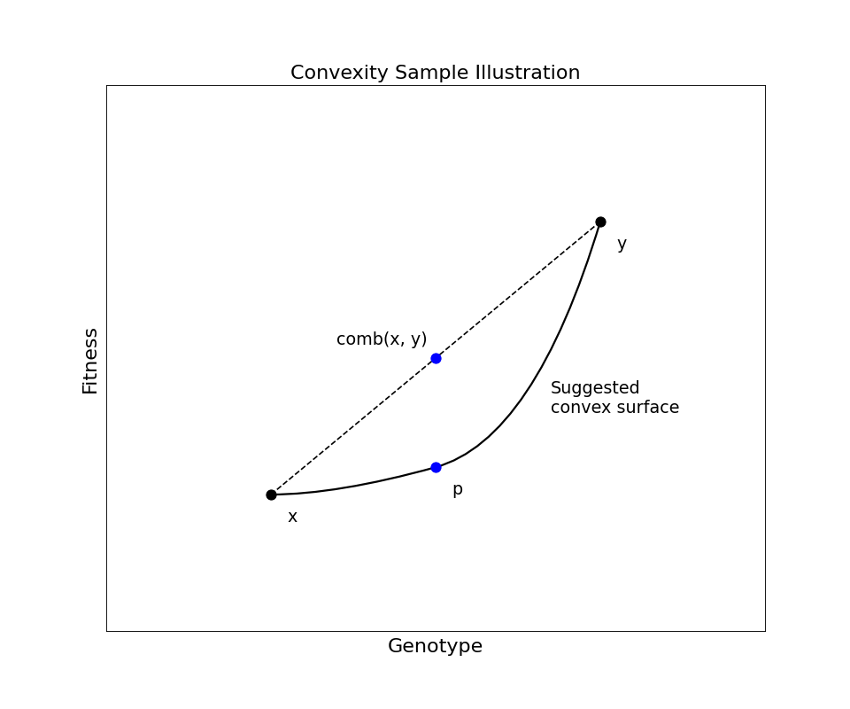
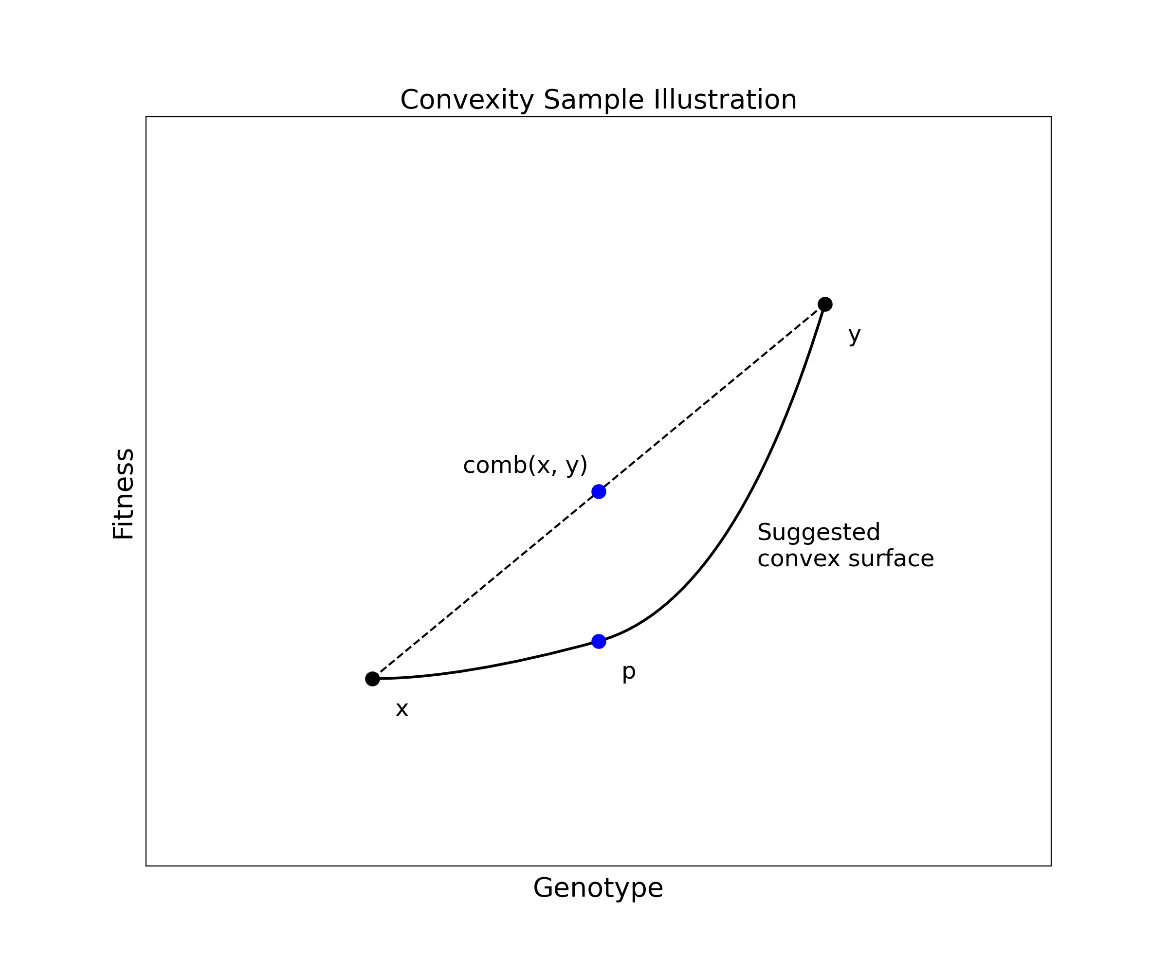
The algorithm used here is best explained by the following graphic:
(Source code, png, hires.png, pdf)

We take a number of random pairs \(x, y\) of individuals from the initial design (sample), and compute a third point \(p\) from them via a convex combination of the original two points (i.e. a random point lying along the line between the original points). Then we compare the fitness \(f(p)\) of the new point to the fitness that the point would have if the landscape were perfectly linear between the original points. That is, we compute the difference between the complex combination of the parents’ fitness values \(f(x)\) and \(f(y)\) and the fitness value of their genomes’ complex combination, \(f(p)\).
\[\delta = f(p) - \text{comb}(f(x), f(y))\]When \(\delta \approx 0\), it suggests local linearity of the fitness landscape, whereas when \(\delta < 0\), convexity is suggested.
To compute these features, we’ll need a problem and a representation:
>>> from leap_ec.decoder import IdentityDecoder
>>> from leap_ec.individual import Individual
>>> from leap_ec.representation import Representation
>>> from leap_ec.real_rep import initializers, problems
>>> DIMENSIONS = 10
>>> N_SAMPLES = 50*DIMENSIONS
>>> problem = problems.SpheroidProblem()
>>> representation = Representation(
...     initialize=initializers.create_real_vector(bounds=[(-5.12, 5.12)]*DIMENSIONS)
... )
We’ll also need an initial sample of individuals must be provided, with its fitnesses already evaluated:
>>> initial_sample = representation.create_population(N_SAMPLES, problem)
>>> initial_sample = Individual.evaluate_population(initial_sample);
The feature computation uses this as its initial “experiment design,” and then takes additional fitness samples as needed when we call the constructor:
>>> convex = ELAConvexity(problem, representation, design_individuals=initial_sample)
The resulting object can be used to compute the various feature calculations:
>>> x = convex.convex_p()
>>> x = convex.linear_p()
>>> x = convex.linear_deviation()
- property combinations
Contains the list of (f, p) pairs, where f is the convex combination of the fitness pair that was used in the ith test, and p is the individual formed from the convex combination of their genomes.
- convex_p(threshold: float = -1e-10)
Estimate the probability that the landscape is convex by calculating the frequency with which
\[\delta < \tau\]where \(\tau\) is a small negative threshold (typically \(-10^{-10}\)).
- Parameters
threshold (float) – the value of \(\tau\).
- property deltas
Contains the list of \(\delta = f(p) - \text{comb}(f(x), f(y))\) values that were computed for the convexity tests.
- linear_deviation()
Estimate the deviation of the landscape from linearity by averaging the \(\delta\) values.
- linear_deviation_abs()
Estimate the deviation of the landscape of linearity by averagin the absolute value \(|\delta|\) of the computed deltas.
Sometimes this is simply the negative of linear_deviation() (ex. when the function is completely convex), but other times the two values differ considerably.
- linear_p(threshold: float = -1e-10)
Estimate the probability that the landscape is linear by calculating the frequency with which
\[| \delta | < \tau\]where \(\tau\) is a small negative threshold (typically \(-10^{-10}\)).
- Parameters
threshold (float) – the value of \(\tau\).
- property pairs
Contains all of the pairs of original individuals that were used in the convexity tests.
- results_table(function_name=None)
Return a Pandas dataframe as a convenience, with one row for each computed feature.
Module contents
This package contains algorithms for computing statistical properties of landscapes.
Much of the research on landscape features is focused on understanding why some problems are easy or hard to solve for certain algorithms, or on how we might use statistical features to train machine learning models to assist in algorithm selection.
For a good survey of the field, look to the following paper:
Malan, Katherine Mary. “A Survey of Advances in Landscape Analysis for Optimisation.” Algorithms 14.2 (2021): 40.