Probes
Probes are special pipeline operators that can be used to echo state of passing individuals or other data. For example, you might want to print the state of an individual with two probes, one before a mutation operator is applied, and another afterwards to observe the effects of mutation.
These are probes do more than passive reporting of data that passes through the pipeline – they actually do some data processing and report that.
Probes are pipeline operators to instrument state that passes through the pipeline such as populations or individuals.
- class leap_ec.probe.AttributesCSVProbe(attributes=(), stream=<_io.TextIOWrapper name='<stdout>' mode='w' encoding='UTF-8'>, do_dataframe=False, best_only=False, header=True, do_fitness=False, do_genome=False, notes=None, extra_metrics=None, job=None, context={'leap': {'distrib': {'non_viable': 0}, 'generation': 100}})
An operator that records the specified attributes for all the individuals (or just the best individual) in population in CSV-format to the specified stream and/or to a DataFrame.
- Parameters
attributes – list of attribute names to record, as found in the individuals’ attributes field
stream – a file object to write the CSV rows to (defaults to sys.stdout). Can be None if you only want a DataFrame
do_dataframe (bool) – if True, data will be collected in memory as a Pandas DataFrame, which can be retrieved by calling the dataframe property after (or during) the algorithm run. Defaults to False, since this can consume a lot of memory for long-running algorithms.
best_only (bool) – if True, attributes will only be recorded for the best-fitness individual; otherwise a row is recorded for every individual in the population
header (bool) – if True (the default), a CSV header is printed as the first row with the column names
do_fitness (bool) – if True, the individuals’ fitness is included as one of the columns
do_genomes (bool) – if True, the individuals’ genome is included as one of the columns
notes (str) – a dict of optional constant-value columns to include in all rows (ex. to identify and experiment or parameters)
extra_metrics – a dict of ‘column_name’: function pairs, to compute optional extra columns. The functions take a the population as input as a list of individuals, and their return value is printed in the column.
job (int) – a job ID that will be included as a constant-value column in all rows (ex. typically an integer, indicating the ith run out of many)
context – the algorithm context we use to read the current generation from (so we can write it to a column)
Individuals contain some build-in attributes (namely fitness, genome), and also a dict of additional custom attributes called, well, attributes. This class allows you to log all of the above.
Most often, you will want to record only the best individual in the population at each step, and you’ll just want to know its fitness and genome. You can do this with this class’s boolean flags. For example, here’s how you’d record the best individual’s fitness and genome to a dataframe:
>>> from leap_ec.global_vars import context
>>> from leap_ec.data import test_population
>>> probe = AttributesCSVProbe(do_dataframe=True, best_only=True,
...                            do_fitness=True, do_genome=True)
>>> context['leap']['generation'] = 100
>>> probe(test_population) == test_population
True
You can retrieve the result programatically from the dataframe property:
>>> probe.dataframe
   step  fitness           genome
0   100        4  [0, 1, 1, 1, 1]
By default, the results are also written to sys.stdout. You can pass any file object you like into the stream parameter.
Another common use of this task is to record custom attributes that are stored on individuals in certain kinds of experiments. Here’s how you would record the values of ind.foo and ind.bar for every individual in the population. We write to a stream object this time to demonstrate how to use the probe without a dataframe:
>>> import io
>>> stream = io.StringIO()
>>> probe = AttributesCSVProbe(attributes=['foo', 'bar'], stream=stream)
>>> context['leap']['generation'] = 100
>>> r = probe(test_population)
>>> print(stream.getvalue())
step,foo,bar
100,GREEN,Colorless
100,15,green
100,BLUE,ideas
100,72.81,sleep
- property dataframe
Property for retrieving a Pandas DataFrame representation of the collected data.
- get_row_dict(ind)
Compute a full row of data from a given individual.
- class leap_ec.probe.BestSoFarIterProbe(stream=<_io.TextIOWrapper name='<stdout>' mode='w' encoding='UTF-8'>, header=True, context={'leap': {'distrib': {'non_viable': 0}, 'generation': 100}})
- This probe takes an iterator as input and will track the
best-so-far (BSF) individual in the all the individuals it sees.
Insert an object of this class into a pipeline to have it track the the best individual it sees so far. It will write the current best individual for each __call__ invocation to a given stream in CSV format.
Like many operators, this operator checks the context object to retrieve the current generation number for output purposes.
>>> from leap_ec import context, data
>>> from leap_ec import probe
>>> pop = data.test_population
>>> context['leap']['generation'] = 12
The probe will write its output to the provided stream (default is stdout, but we illustrate here with a StringIO stream):
>>> import io
>>> stream = io.StringIO()
>>> probe = BestSoFarIterProbe(stream=stream)
>>> bsf_output_iter = probe(iter(pop))
>>> x = next(bsf_output_iter)
>>> x = next(bsf_output_iter)
>>> x = next(bsf_output_iter)
>>> print(stream.getvalue())
step,bsf
12,...
12,...
12,...
- class leap_ec.probe.BestSoFarProbe(stream=<_io.TextIOWrapper name='<stdout>' mode='w' encoding='UTF-8'>, header=True, context={'leap': {'distrib': {'non_viable': 0}, 'generation': 100}})
- This probe takes an list of individuals as input and will track the
best-so-far (BSF) individual across all the population it has seen.
Insert an object of this class into a pipeline to have it track the the best individual it sees so far. It will write the current best individual for each __call__ invocation to a given stream in CSV format.
Like many operators, this operator checks the context object to retrieve the current generation number for output purposes.
>>> from leap_ec import context, data
>>> from leap_ec import probe
>>> pop = data.test_population
>>> context['leap']['generation'] = 12
The probe will write its output to the provided stream (default is stdout, but we illustrate here with a StringIO stream):
>>> import io
>>> stream = io.StringIO()
>>> probe = BestSoFarProbe(stream=stream)
>>> new_pop = probe(pop)
>>> print(stream.getvalue())
step,bsf
12,4
This operator does not change the state of the population: >>> new_pop == pop True
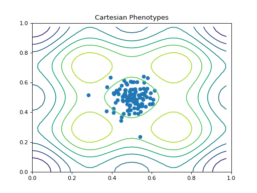
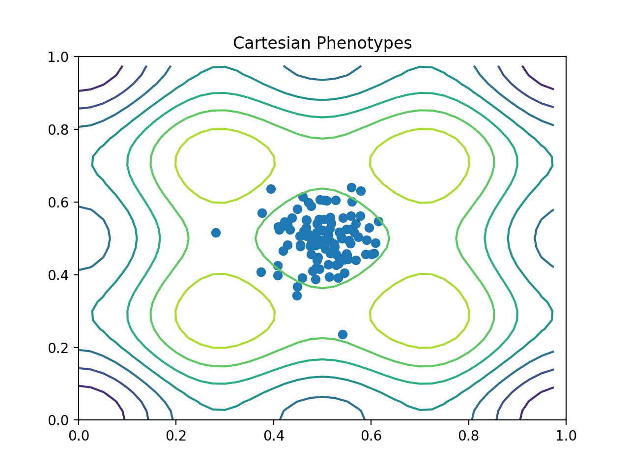
- class leap_ec.probe.CartesianPhenotypePlotProbe(ax=None, xlim=(-5.12, 5.12), ylim=(-5.12, 5.12), contours=None, granularity=None, title='Cartesian Phenotypes', modulo=1, context={'leap': {'distrib': {'non_viable': 0}, 'generation': 100}}, pad=())
Measure and plot a scatterplot of the populations’ location in a 2-D phenotype space.
- Parameters
ax (Axes) – Matplotlib axes to plot to (if None, a new figure will be created).
xlim ((float, float)) – Bounds of the horizontal axis.
ylim ((float, float)) – Bounds of the vertical axis.
contours (Problem) – a problem defining a 2-D fitness function (this will be used to draw fitness contours in the background of the scatterplot).
granularity (float) – (Optional) spacing of the grid to sample points along while drawing the fitness contours. If none is given, then the granularity will default to 1/50th of the range of the function’s bounds attribute.
modulo (int) – take and plot a measurement every modulo steps ( default 1).
pad – A list of extra gene values, used to fill in the hidden dimensions with contants while drawing fitness contours.
Attach this probe to matplotlib
Axesand then insert it into an EA’s operator pipeline to get a live phenotype plot that updates every modulo steps.>>> import matplotlib.pyplot as plt >>> from leap_ec.probe import CartesianPhenotypePlotProbe >>> from leap_ec.representation import Representation
>>> from leap_ec.individual import Individual
>>> from leap_ec.algorithm import generational_ea
>>> from leap_ec import ops
>>> from leap_ec.decoder import IdentityDecoder
>>> from leap_ec.real_rep.problems import CosineFamilyProblem
>>> from leap_ec.real_rep.initializers import create_real_vector
>>> from leap_ec.real_rep.ops import mutate_gaussian
>>> # The fitness landscape
>>> problem = CosineFamilyProblem(alpha=1.0, global_optima_counts=[2, 2], local_optima_counts=[2, 2])
>>> # If no axis is provided, a new figure will be created for the probe to write to
>>> trajectory_probe = CartesianPhenotypePlotProbe(contours=problem,
...                                        xlim=(0, 1), ylim=(0, 1),
...                                        granularity=0.025)
>>> # Create an algorithm that contains the probe in the operator pipeline
>>> pop_size = 100
>>> ea = generational_ea(max_generations=20, pop_size=pop_size,
...                      problem=problem,
...
...                      representation=Representation(
...                         individual_cls=Individual,
...                         initialize=create_real_vector(bounds=[[0.4, 0.6]] * 2),
...                         decoder=IdentityDecoder()
...                      ),
...
...                      pipeline=[
...                         trajectory_probe,  # Insert the probe into the pipeline like so
...                         ops.tournament_selection,
...                         ops.clone,
...                         mutate_gaussian(std=0.05, expected_num_mutations='isotropic', bounds=(0, 1)),
...                         ops.evaluate,
...                         ops.pool(size=pop_size)
...                      ])
>>> result = list(ea);
(Source code, png, hires.png, pdf)

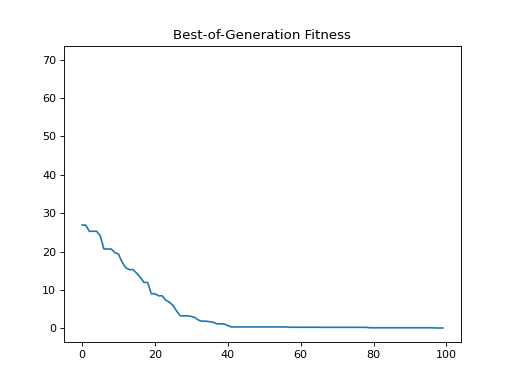
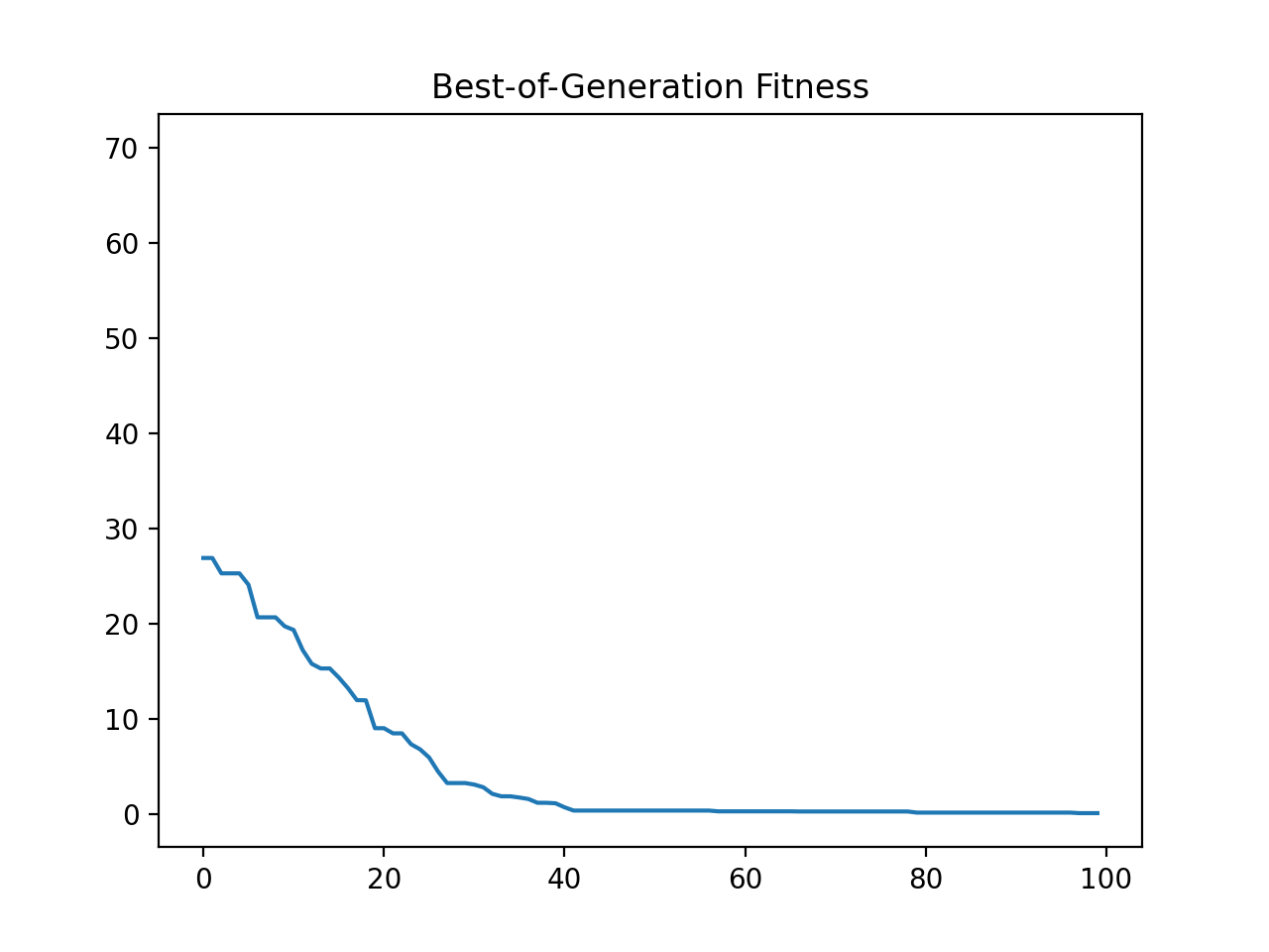
- class leap_ec.probe.FitnessPlotProbe(ax=None, xlim=None, ylim=None, modulo=1, title='Best-of-Generation Fitness', x_axis_value=None, context={'leap': {'distrib': {'non_viable': 0}, 'generation': 100}})
Measure and plot a population’s fitness trajectory.
- Parameters
ax (Axes) – Matplotlib axes to plot to (if None, a new figure will be created).
xlim ((float, float)) – Bounds of the horizontal axis.
ylim ((float, float)) – Bounds of the vertical axis.
modulo (int) – take and plot a measurement every modulo steps ( default 1).
title – title to print on the plot
x_axis_value – optional function to define what value gets plotted on the x axis. Defaults to pulling the ‘generation’ value out of the default context object.
context – set a context object to query for the current generation. Defaults to the standard leap_ec.context object.
Attach this probe to matplotlib
Axesand then insert it into an EA’s operator pipeline.>>> import matplotlib.pyplot as plt >>> from leap_ec.probe import FitnessPlotProbe >>> from leap_ec.representation import Representation
>>> f = plt.figure()  # Setup a figure to plot to
>>> plot_probe = FitnessPlotProbe(ylim=(0, 70), ax=plt.gca())
>>> # Create an algorithm that contains the probe in the operator pipeline
>>> from leap_ec.individual import Individual
>>> from leap_ec.decoder import IdentityDecoder
>>> from leap_ec import ops
>>> from leap_ec.real_rep.problems import SpheroidProblem
>>> from leap_ec.real_rep.ops import mutate_gaussian
>>> from leap_ec.real_rep.initializers import create_real_vector
>>> from leap_ec.algorithm import generational_ea
>>> l = 10
>>> pop_size = 10
>>> ea = generational_ea(max_generations=100, pop_size=pop_size,
...                      problem=SpheroidProblem(maximize=False),
...
...                      representation=Representation(
...                         individual_cls=Individual,
...                         decoder=IdentityDecoder(),
...                         initialize=create_real_vector(bounds=[[-5.12, 5.12]] * l)
...                      ),
...
...                      pipeline=[
...                         plot_probe,  # Insert the probe into the pipeline like so
...                         ops.tournament_selection,
...                         ops.clone,
...                         mutate_gaussian(std=0.2, expected_num_mutations='isotropic'),
...                         ops.evaluate,
...                         ops.pool(size=pop_size)
...                      ])
>>> result = list(ea);
(Source code, png, hires.png, pdf)

To get a live-updated plot that words like a real-time video of the EA’s progress, use this probe in conjunction with the %matplotlib notebook magic for Jupyter Notebook (as opposed to %matplotlib inline, which only allows static plots).
- class leap_ec.probe.FitnessStatsCSVProbe(stream=<_io.TextIOWrapper name='<stdout>' mode='w' encoding='UTF-8'>, header=True, extra_metrics=None, comment=None, job: ~typing.Optional[str] = None, notes: ~typing.Optional[~typing.Dict] = None, modulo: int = 1, context: ~typing.Dict = {'leap': {'distrib': {'non_viable': 0}, 'generation': 100}})
A probe that records basic fitness statistics for a population to a text stream in CSV format.
This is meant to capture the “bread and butter” values you’ll typically want to see in any population-based optimization experiment. If you want additional columns with custom values, you can pass in a dict of notes with constant values or extra_metrics with functions to compute them.
- Parameters
stream – the file object to write to (defaults to sys.stdout)
header – whether to print column names in the first line
extra_metrics – a dict of ‘column_name’: function pairs, to compute optional extra columns. The functions take a the population as input as a list of individuals, and their return value is printed in the column.
job – optional constant job ID, which will be printed as the first column
notes (str) – a dict of optional constant-value columns to include in all rows (ex. to identify and experiment or parameters)
context – a LEAP context object, used to retrieve the current generation from the EA state (i.e. from context[‘leap’][‘generation’])
In this example, we’ll set up two three inputs for the probe: an output stream, the generation number, and a population.
We use a StringIO stream to print the results here, but in practice you often want to use sys.stdout (the default) or a file object:
>>> import io
>>> stream = io.StringIO()
The probe also relies on LEAP’s algorithm context to determine the generation number:
>>> from leap_ec.global_vars import context
>>> context['leap']['generation'] = 100
Here’s how we’d compute fitness statistics for a test population. The population is unmodified:
>>> from leap_ec.data import test_population
>>> probe = FitnessStatsCSVProbe(stream=stream, job=15, notes={'description': 'just a test'})
>>> probe(test_population) == test_population
True
and the output has the following columns: >>> print(stream.getvalue()) job, description, step, bsf, mean_fitness, std_fitness, min_fitness, max_fitness 15, just a test, 100, 4, 2.5, 1.11803…, 1, 4 <BLANKLINE>
To add custom columns, use the extra_metrics dict. For example, here’s a function that computes the median fitness value of a population:
>>> import numpy as np
>>> median = lambda p: np.median([ ind.fitness for ind in p ])
We can include it in the fitness stats report like so:
>>> stream = io.StringIO()
>>> extras_probe = FitnessStatsCSVProbe(stream=stream, job="15", extra_metrics={'median_fitness': median})
>>> extras_probe(test_population) == test_population
True
>>> print(stream.getvalue())
job, step, bsf, mean_fitness, std_fitness, min_fitness, max_fitness, median_fitness
15, 100, 4, 2.5, 1.11803..., 1, 4, 2.5
- comment_character = '#'
- default_metric_cols = ('bsf', 'mean_fitness', 'std_fitness', 'min_fitness', 'max_fitness')
- time_col = 'step'
- write_comment(stream)
- write_header(stream)
- class leap_ec.probe.HeatMapPhenotypeProbe(ax=None, title='HeatMap of Phenotypes', modulo=1, context={'leap': {'distrib': {'non_viable': 0}, 'generation': 100}})
- class leap_ec.probe.HistPhenotypePlotProbe(ax=None, title='Histogram of Phenotypes', modulo=1, context={'leap': {'distrib': {'non_viable': 0}, 'generation': 100}})
A visualization probe that uses matplotlib to show a live histogram of the population’s phenotypes.
This typically makes the most since for 1-dimensional genotypes.
- class leap_ec.probe.PopulationMetricsPlotProbe(ax=None, metrics=None, xlim=None, ylim=None, modulo=1, title='Population Metrics', x_axis_value=None, context={'leap': {'distrib': {'non_viable': 0}, 'generation': 100}})
- reset()
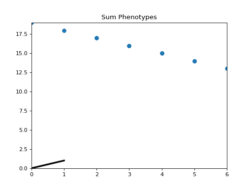
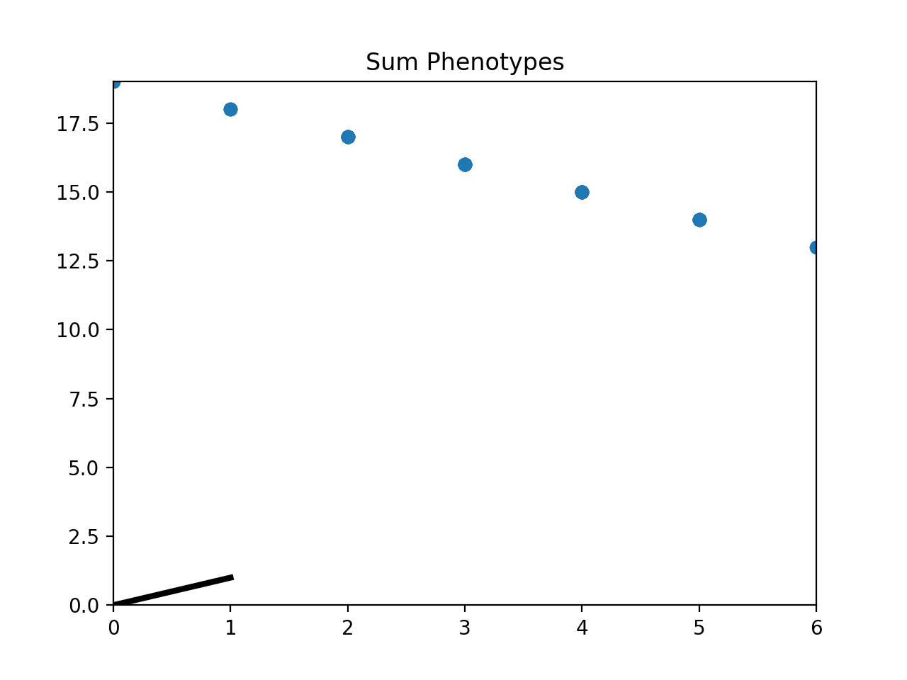
- class leap_ec.probe.SumPhenotypePlotProbe(ax=None, xlim=(-5.12, 5.12), ylim=(-5.12, 5.12), problem=None, granularity=1, title='Sum Phenotypes', modulo=1, context={'leap': {'distrib': {'non_viable': 0}, 'generation': 100}})
Plot the population’s location on a fitness landscape that is defined over the sum of a vector phenotype’s elements. This is useful for visualizing OneMax functions and similar functions that can be understood in terms of a graph with “the number of ones” along the x axis.
- Parameters
ax (Axes) – Matplotlib axes to plot to (if None, a new figure will be created).
xlim ((float, float)) – Bounds of the horizontal axis.
ylim ((float, float)) – Bounds of the vertical axis.
problem (Problem) – a problem that will be used to draw a fitness curve.
granularity (float) – (Optional) spacing of the grid to sample points along while drawing the fitness contours. If none is given, then the granularity will default to 1.0.
modulo (int) – take and plot a measurement every modulo steps ( default 1).
Attach this probe to matplotlib
Axesand then insert it into an EA’s operator pipeline to get a live phenotype plot that updates every modulo steps.>>> import matplotlib.pyplot as plt >>> from leap_ec.probe import SumPhenotypePlotProbe >>> from leap_ec.representation import Representation
>>> from leap_ec.individual import Individual
>>> from leap_ec.algorithm import generational_ea
>>> from leap_ec import ops
>>> from leap_ec.binary_rep.problems import DeceptiveTrap
>>> from leap_ec.binary_rep.initializers import create_binary_sequence
>>> from leap_ec.binary_rep.ops import mutate_bitflip
>>> # The fitness landscape
>>> problem = DeceptiveTrap()
>>> # If no axis is provided, a new figure will be created for the probe to write to
>>> dimensions = 20
>>> trajectory_probe = SumPhenotypePlotProbe(problem=problem,
...                                        xlim=(0, dimensions), ylim=(0, dimensions))
>>> # Create an algorithm that contains the probe in the operator pipeline
>>> pop_size = 100
>>> ea = generational_ea(max_generations=20, pop_size=pop_size,
...                      problem=problem,
...
...                      representation=Representation(
...                         individual_cls=Individual,
...                         initialize=create_binary_sequence(length=dimensions)
...                      ),
...
...                      pipeline=[
...                         trajectory_probe,  # Insert the probe into the pipeline like so
...                         ops.tournament_selection,
...                         ops.clone,
...                         mutate_bitflip(expected_num_mutations=1),
...                         ops.evaluate,
...                         ops.pool(size=pop_size)
...                      ])
>>> result = list(ea);
(Source code, png, hires.png, pdf)
- leap_ec.probe.best_of_gen(population)
Syntactic sugar to select the best individual in a population.
- Parameters
population – a list of individuals
context – optional dict of auxiliary state (ignored)
>>> from leap_ec.data import test_population
>>> print(best_of_gen(test_population))
Individual<...> with fitness 4
- leap_ec.probe.num_fixated_metric(population: list)
Computes the genetic diversity of the population by counting the number of variables in the genome that have zero variance.
This is a so-called “column-wise” metric, in the sense that it considers each element of the solution vectors independently.
- leap_ec.probe.pairwise_squared_distance_metric(population: list)
Computes the genetic diversity of a population by considering the sum of squared Euclidean distances between individual genomes.
We compute this in \(O(n)\) by writing the sum in terms of distance from the population centroid \(c\):
\[\mathcal{D}(\text{population}) = \sum_{i=1}^n \sum_{j=1}^n \| x_i - x_j \|^2 = 2n \sum_{i=1}^n \| x_i - c \|^2\]
- leap_ec.probe.print_individual(next_individual: ~typing.Iterator = '__no__default__', prefix='', stream=<_io.TextIOWrapper name='<stdout>' mode='w' encoding='UTF-8'>) Iterator
Just echoes the individual from within the pipeline
Uses next_individual.__str__
- Parameters
next_individual – iterator for next individual to be printed
prefix – prefix appended to the start of the line
stream – File object passed to print
- Returns
the same individual, unchanged
- leap_ec.probe.print_population(population, generation)
Convenience function for pretty printing a population that’s associated with a given generation
- Parameters
population – The population of individuals to be printed
generation – The generation of the population
- Returns
None
- leap_ec.probe.print_probe(population='__no__default__', probe='__no__default__', stream=<_io.TextIOWrapper name='<stdout>' mode='w' encoding='UTF-8'>, prefix='')
pipeline operator for printing the given population
This is really a wrapper around probe that, itself, gets passed te entire population.
The optional prefix is used to tag the output. For example, you may want to print ‘before’ to indicate that the population is before an operator is applied.
- Parameters
population – to be printed
probe – secondary probe that gets the poplation as input and for which the output is passed to stream
stream – to write output
prefix – optional string prefix to prepend to output
- Returns
population
- leap_ec.probe.sum_of_variances_metric(population: list)
Computes the genetic diversity of a population by considering the sum of the variances of each variable in the genome.
\[\mathcal{D}(\text{population}) = \sum_{i=1}^L \mathbb{E}_{j \in P}\left[ x_j[i] - \mathbb{E}[x_j[i]] \right]\]This is a so-called “column-wise” metric, in the sense that it considers each element of the solution vectors independently.