Problems

This section covers Problem classes in more detail.

Class Summary

_images/problem_class_diagram.svg — Fig. 7 **The `Problem` abstract-base class** This class diagram shows the detail for Problem, which is an abstract base class (ABC). It has three abstract methods that must be over-ridden by subclasses. evaluate() takes a phenome from an individual and compute a fitness from that. worse_than() and equivalent() compare fitnesses from two different individuals and, as the name suggests, respectively returns the worst of the two or the equivalent within the Problem context.

As shown in Fig. 7, the Problem abstract-base class has three abstract methods. evaluate() takes a phenome that was decode()d from an Individual’s genome, and returns a value denoting the quality, or fitness, of that individual. Problems are also used to compare the fitnesses between Individuals. worse_than() returns true if the first individual is less fit than the second. Similarly, equivalent() is used to determine if two given fitnesses are effectively the same.

Class API

Defines the abstract-base classes Problem, ScalarProblem, and FunctionProblem.

class leap_ec.problem.AlternatingProblem(problems, modulo, context={'leap': {'distrib': {'non_viable': 0}}})

equivalent(first_fitness, second_fitness)

evaluate(phenome)

Evaluate the given phenome.

Practitioners must over-ride this member function.

Note that by default the individual comparison operators assume a maximization problem; if this is a minimization problem, then just negate the value when returning the fitness.

Parameters: phenome – the phenome to evaluate (this will not be modified)
Returns: the fitness value

get_current_problem()

worse_than(first_fitness, second_fitness)

class leap_ec.problem.AverageFitnessProblem(wrapped_problem, n: int)

Problem wrapper that copies each genome n times, evaluates them, and averages the results back together to produce a mean-fitness estimate.

This is a common strategy for approaching noisy fitness functions, to make it easier for an optimization algorithm to follow a gradient.

>>> from leap_ec.real_rep.problems import NoisyQuarticProblem
>>> p = AverageFitnessProblem(
...                 wrapped_problem = NoisyQuarticProblem(),
...                 n = 20)
>>> x = [ 1, 1, 1, 1 ]
>>> y = p.evaluate(x)
>>> print(f"Fitness: {y}")  # The mean of this will be approximately 10
Fitness: ...

equivalent(first_fitness, second_fitness)

evaluate(phenome): Evaluates the wrapped function n times sequentially and returns the mean.

evaluate_multiple(phenomes: list): Evaluate a collections of phenomes by creating n jobs for each phenome, sending all the jobs to the wrapped evaluate_multiple() function, and then averaging the n results for each phenome into a list of results.

worse_than(first_fitness, second_fitness)

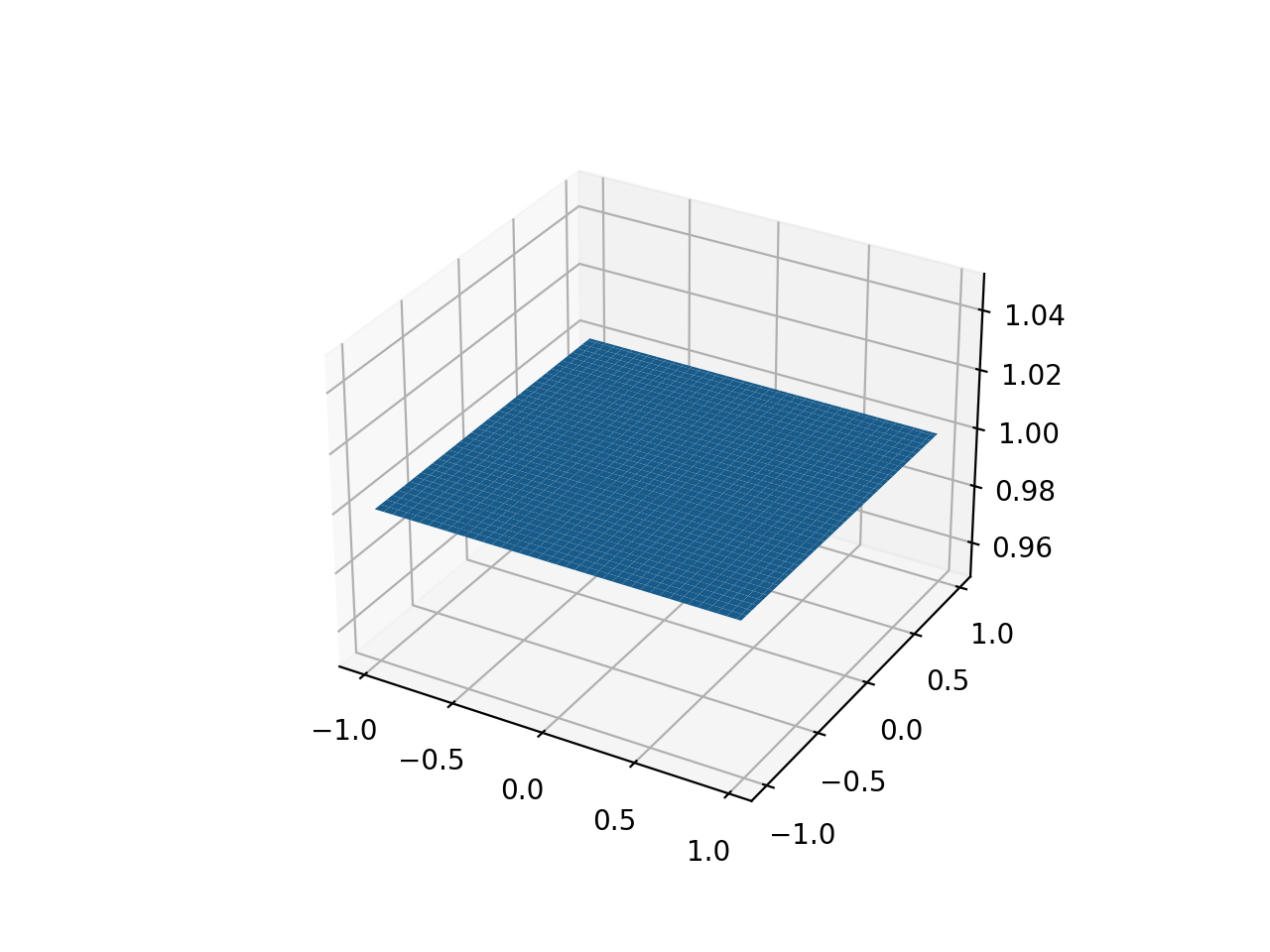
class leap_ec.problem.ConstantProblem(maximize=False, c=1.0)

A flat landscape, where all phenotypes have the same fitness.

This is sometimes useful for sanity checks or as a control in certain kinds of research.

\[f(\vec{x}) = c\]

Parameters: c (float) – the fitness value to return for any input.

from leap_ec.problem import ConstantProblem
from leap_ec.real_rep.problems import plot_2d_problem
bounds = ConstantProblem.bounds
plot_2d_problem(ConstantProblem(), xlim=bounds, ylim=bounds, granularity=0.025)

(Source code, png, hires.png, pdf)

bounds = (-1.0, 1.0)

evaluate(phenome, *args, **kwargs)

Return a contant value for any input phenome:

>>> phenome = [0.5, 0.8, 1.5]
>>> ConstantProblem().evaluate(phenome)
1.0

>>> ConstantProblem(c=500.0).evaluate('foo bar')
500.0

Parameters: phenome – phenome to be evaluated
Returns: 1.0, or the constant defined in the constructor

class leap_ec.problem.CooperativeProblem(wrapped_problem, num_trials: int, collaborator_selector, combined_decoder: ~leap_ec.decoder.Decoder = IdentityDecoder(), log_stream=None, combine_genomes=<function CooperativeProblem.<lambda>>, context={'leap': {'distrib': {'non_viable': 0}}})

A Problem that implements cooperative coevolution. This provides a fitness function that takes partial solutions as input (i.e. from one of the subpopulations of the cooperative algorithm), and evaluates their fitness by combining them with other individuals in the population.

You can think of a CooperativeProblem as defining a fitness function for a subpopulation in a multi-population model, where the fitness function that is computed is itself a function of the state of the other subpopulations:

..math

mbox{fitness} = f_{p_i}(vec{mathbf{x}}, mathcal{P} \ p_i)

This class works by wrapping another fitness function, which is defined over complete solutions, and by taking a selection operator (which is used to select “collaborators” from other subpopulations to form complete solutions):

>>> from leap_ec import ops
>>> from leap_ec.real_rep.problems import SpheroidProblem
>>> complete_problem = SpheroidProblem()
>>> problem = CooperativeProblem(
...             wrapped_problem = SpheroidProblem(),
...             num_trials = 3,
...             collaborator_selector = ops.random_selection)

equivalent(first_fitness, second_fitness)

evaluate(phenome, *args, **kwargs)

Evaluate the given phenome.

Practitioners must over-ride this member function.

Note that by default the individual comparison operators assume a maximization problem; if this is a minimization problem, then just negate the value when returning the fitness.

Parameters: phenome – the phenome to evaluate (this will not be modified)
Returns: the fitness value

evaluate_multiple(phenomes, individuals)

Evaluate multiple phenomes all at once, returning a list of fitness values.

By default this just calls self.evaluate() multiple times. Override this if you need to, say, send a group of individuals off to parallel

worse_than(first_fitness, second_fitness)

class leap_ec.problem.ExternalProcessProblem(command: str, maximize: bool, args: Optional[list] = None)

Evaluate individuals by launching an external program, writing phenomes to its stdin as CSV rows, and reading back fitness values from its stdout.

Assumes that individuals are represented with list phenomes with elements that can be cast to strings.

evaluate(phenome)

Evaluate the given phenome.

Practitioners must over-ride this member function.

Note that by default the individual comparison operators assume a maximization problem; if this is a minimization problem, then just negate the value when returning the fitness.

Parameters: phenome – the phenome to evaluate (this will not be modified)
Returns: the fitness value

evaluate_multiple(phenomes, *args, **kwargs)

Evaluate multiple phenomes all at once, returning a list of fitness values.

By default this just calls self.evaluate() multiple times. Override this if you need to, say, send a group of individuals off to parallel

class leap_ec.problem.FitnessOffsetProblem(problem, fitness_offset, maximize=None)

Takes an existing function and adds a constant value to it output.

\[f'(\mathbf{x}) = f(\mathbf{x}) + c\]

Parameters

problem – the original problem to wrape
fitness_offset (float) – the scalar constant to add

evaluate(phenome)

Evaluates the phenome’s fitness in the wrapped function, then adds the constant.

For example, here the original fitness function returns 5.0, but we subtract 3.5 from it so that it yields 1.5.

>>> original = ConstantProblem(c=5.0)
>>> problem = FitnessOffsetProblem(original, fitness_offset=-3.5)
>>> problem.evaluate([0, 1, 2])
1.5

class leap_ec.problem.FunctionProblem(fitness_function, maximize)

A convenience wrapper that takes a vanilla function that returns scalar fitness values and makes it usable as an objective function.

evaluate(phenome, *args, **kwargs)

Evaluate the given phenome.

Practitioners must over-ride this member function.

Note that by default the individual comparison operators assume a maximization problem; if this is a minimization problem, then just negate the value when returning the fitness.

Parameters: phenome – the phenome to evaluate (this will not be modified)
Returns: the fitness value

class leap_ec.problem.Problem

Abstract Base Class used to define problem definitions.

A Problem is in charge of two major parts of an EA’s behavior:

Fitness evaluation (the evaluate() method)

Fitness comparision (the worse_than() and equivalent() methods)

abstract equivalent(first_fitness, second_fitness)

abstract evaluate(phenome, *args, **kwargs)

Evaluate the given phenome.

Practitioners must over-ride this member function.

Note that by default the individual comparison operators assume a maximization problem; if this is a minimization problem, then just negate the value when returning the fitness.

Parameters: phenome – the phenome to evaluate (this will not be modified)
Returns: the fitness value

evaluate_multiple(phenomes)

Evaluate multiple phenomes all at once, returning a list of fitness values.

By default this just calls self.evaluate() multiple times. Override this if you need to, say, send a group of individuals off to parallel

abstract worse_than(first_fitness, second_fitness)

class leap_ec.problem.ScalarProblem(maximize)

A problem that compares individuals based on their scalar fitness values.

Inherit from this class and implement the evaluate() method to implement an objective function that returns a single real-valued fitness value.

equivalent(first_fitness, second_fitness)

Used in Individual.__eq__().

By default returns first.fitness== second.fitness. Please over-ride if this does not hold for your problem.

Returns: true if the first individual is equal to the second

worse_than(first_fitness, second_fitness)

Used in Individual.__lt__().

By default returns first_fitness < second_fitness if a maximization problem, else first_fitness > second_fitness if a minimization problem. Please over-ride if this does not hold for your problem.

Returns: true if the first individual is less fit than the second

leap_ec.problem.concat_combine(collaborators)

Combine a list of individuals by concatenating their genomes.

This is a convenience function intended for use with CooperativeProblem.

Binary Problems API

Inheritance diagram of leap_ec.binary_rep.problems

A set of standard EA problems that rely on a binary-representation

class leap_ec.binary_rep.problems.DeceptiveTrap(maximize=True)

A simple bi-modal function whose global optimum is the Boolean vector of all 1’s, but in which fitness decreases as the number of 1’s in the vector increases—giving it a local optimum of [0, …, 0] with a very wide basin of attraction.

evaluate(phenome)

>>> import numpy as np
>>> p = DeceptiveTrap()

The trap function has a global maximum when the number of one’s is maximized:

>>> p.evaluate(np.array([1, 1, 1, 1, 1, 1, 1, 1, 1, 1]))
10

It’s minimized when we have just one zero: >>> p.evaluate(np.array([1, 1, 1, 1, 0, 1, 1, 1, 1, 1])) 0

And has a local optimum when we have no ones at all: >>> p.evaluate(np.array([0, 0, 0, 0, 0, 0, 0, 0, 0, 0])) 9

class leap_ec.binary_rep.problems.ImageProblem(path, maximize=True, size=(100, 100))

A variation on max_ones that uses an external image file to define a binary target pattern.

evaluate(phenome)

Evaluate the given phenome.

Practitioners must over-ride this member function.

Note that by default the individual comparison operators assume a maximization problem; if this is a minimization problem, then just negate the value when returning the fitness.

Parameters: phenome – the phenome to evaluate (this will not be modified)
Returns: the fitness value

class leap_ec.binary_rep.problems.LeadingOnes(target_string=None, maximize=True)

Implementation of the classic leading-ones problem, where the individuals are represented by a bit vector.

By default, the number of consecutve 1’s starting from the beginning of the phenome are maximized:

>>> p = LeadingOnes()

But an optional target string can also be specified, in which case the number of matches to the target are maximized:

>>> import numpy as np
>>> p = LeadingOnes(target_string=np.array([1, 1, 0, 1, 1, 0, 0, 0 ,0]))

evaluate(phenome)

By default this counts the number of consecutive 1’s at the start of the string:

>>> import numpy as np
>>> p = LeadingOnes()
>>> p.evaluate(np.array([1, 1, 1, 1, 0, 1, 0, 1, 1]))
4

Or, if a target string was given, we count matches:

>>> p = LeadingOnes(target_string=np.array([1, 1, 0, 1, 1, 0, 0, 0 ,0]))
>>> p.evaluate(np.array([1, 1, 1, 1, 0, 1, 0, 1, 1]))
2

class leap_ec.binary_rep.problems.MaxOnes(target_string=None, maximize=True)

Implementation of the classic max-ones problem, where the individuals are represented by a bit vector.

By default, the number of 1’s in the phenome are maximized.

>>> p = MaxOnes()

But an optional target string can also be specified, in which case the number of matches to the target are maximized:

>>> import numpy as np
>>> p = MaxOnes(target_string=np.array([1, 1, 1, 1, 1, 0, 0, 0 ,0]))

evaluate(phenome)

By default this counts the number of 1’s:

>>> from leap_ec.individual import Individual
>>> import numpy as np
>>> p = MaxOnes()
>>> p.evaluate(np.array([0, 0, 1, 1, 0, 1, 0, 1, 1]))
5

Or, if a target string was given, we count matches:

>>> from leap_ec.individual import Individual
>>> import numpy as np
>>> p = MaxOnes(target_string=np.array([1, 1, 1, 1, 1, 0, 0, 0 ,0]))
>>> p.evaluate(np.array([0, 0, 1, 1, 0, 1, 0, 1, 1]))
3

class leap_ec.binary_rep.problems.TwoMax(maximize=True)

A simple bi-modal function that returns the number of 1’s if there are more 1’s than 0’s, else the number of 0’s.

Also known as the “Twin-Peaks” problem.

evaluate(phenome)

>>> import numpy as np
>>> p = TwoMax()

The TwoMax problems returns the number over 1’s if they are in the majority:

>>> p.evaluate(np.array([1, 1, 1, 1, 1, 1, 1, 0, 0, 0]))
7

Else the number of zeros: >>> p.evaluate(np.array([0, 0, 0, 1, 0, 0, 0, 1, 1, 1])) 6

Real-value Problems API

Inheritance diagram of leap_ec.real_rep.problems

This module contains a variety of classic real-valued optimization problems that frequently occur in research benchmarks.

It also contains helpers for translating, rotating, and visualizing them.

class leap_ec.real_rep.problems.AckleyProblem(a=20, b=0.2, c=6.283185307179586, maximize=False)

\[f(\mathbf{x}) = -a \exp \left( -b \sqrt {\frac{1}{d} \sum_{i=1}^d x_i^2} \right) - \exp \left( \frac{1}{d} \sum_{i=1}^d \cos(cx_i) \right) + a + \exp(1)\]

Parameters

a (float) – depth parameter for the bowl-shaped macrostructure
b (float) – exponential scale parameter for the bowl
c (float) – wavenumber (frequency) of the cosine pattern of local optima
maximize (bool) – the function is maximized if True, else minimized.

from leap_ec.real_rep.problems import AckleyProblem, plot_2d_problem
import math
problem = AckleyProblem(a=20, b=0.2, c=2*math.pi)
bounds = AckleyProblem.bounds  # Contains traditional bounds
plot_2d_problem(problem, xlim=bounds, ylim=bounds, granularity=0.25)

(Source code, png, hires.png, pdf)

bounds = [-32.768, 32.768]

evaluate(phenome)

Computes the function value from a real-valued phenome.

Parameters: phenome – real-valued vector to be evaluated
Returns: its fitness.

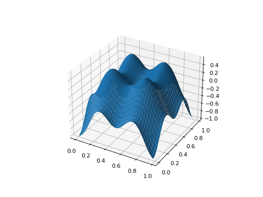
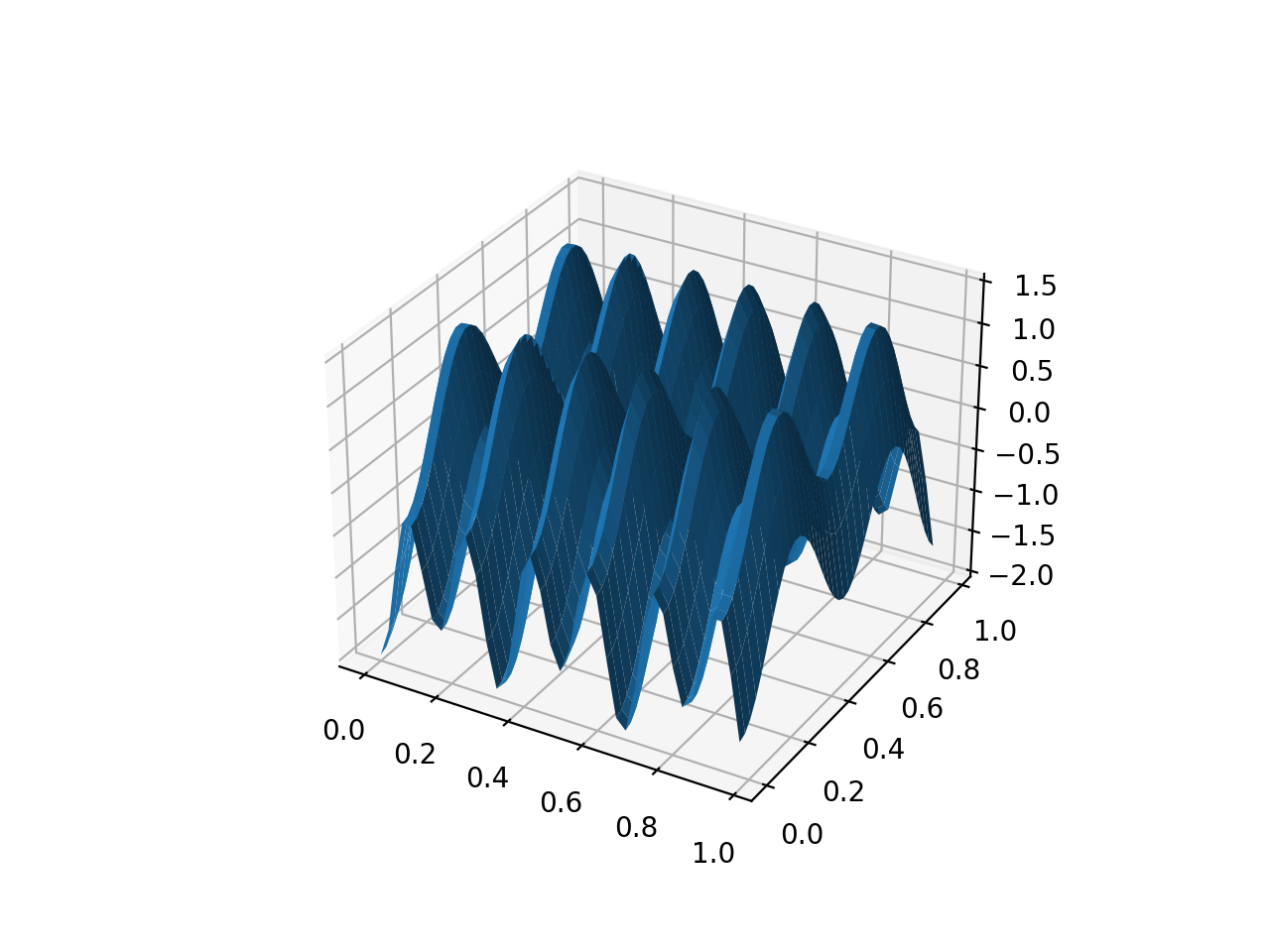
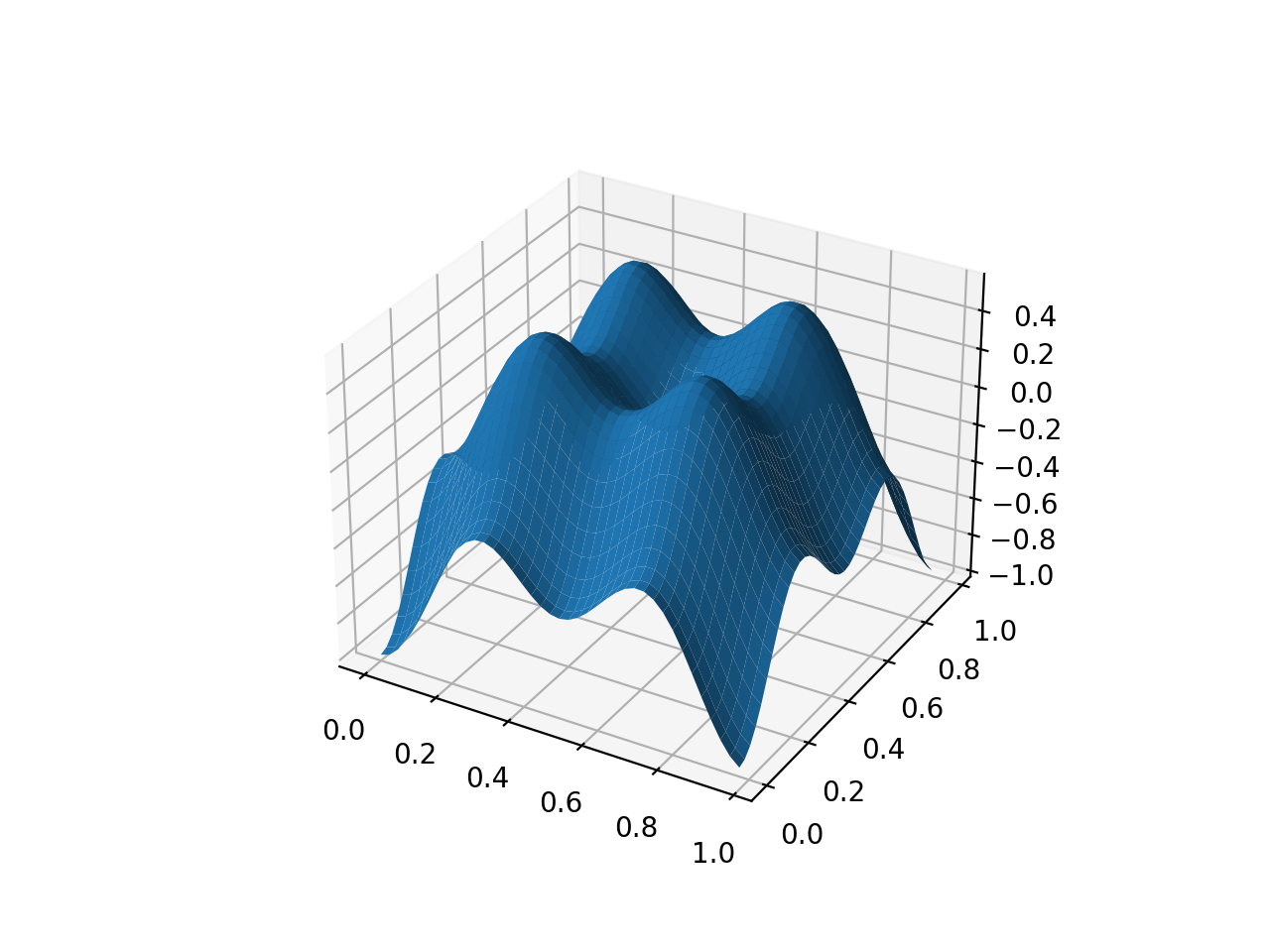
class leap_ec.real_rep.problems.CosineFamilyProblem(alpha, global_optima_counts, local_optima_counts, maximize=False)

A configurable multi-modal function based on combinations of cosines, taken from the problem generators proposed by Rönkkönen et al. [RonkkonenLKL08].

\[f_{\cos}(\mathbf{x}) = \frac{\sum_{i=1}^n -\cos((G_i - 1)2 \pi x_i) - \alpha \cdot \cos((G_i - 1)2 \pi L_i x_i)}{2n}\]

where \(G_i\) and \(L_i\) are parameters that indicate the number of global and local optima, respectively, in the ith dimension.

Parameters

alpha (float) – parameter that controls the depth of the local optima.
global_optima_counts ([int]) – list of integers indicating the number of global optima for each dimension.
local_optima_counts ([int]) – list of integers indicated the number of local optima for each dimension.
maximize – the function is maximized if True, else minimized.

from leap_ec.real_rep.problems import CosineFamilyProblem, plot_2d_problem
problem = CosineFamilyProblem(alpha=1.0, global_optima_counts=[2, 2], local_optima_counts=[2, 2])
bounds = CosineFamilyProblem.bounds  # Contains traditional bounds
plot_2d_problem(problem, xlim=bounds, ylim=bounds, granularity=0.025)

(Source code, png, hires.png, pdf)

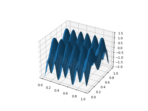
The number of optima can be varied independently by each dimension:

from leap_ec.real_rep.problems import CosineFamilyProblem, plot_2d_problem
problem = CosineFamilyProblem(alpha=3.0, global_optima_counts=[4, 2], local_optima_counts=[2, 2])
bounds = CosineFamilyProblem.bounds  # Contains traditional bounds
plot_2d_problem(problem, xlim=bounds, ylim=bounds, granularity=0.025)

(Source code, png, hires.png, pdf)

bounds = (0, 1)

evaluate(phenome)

Computes the function value from a real-valued phenome.

Parameters: phenome – phenome with a real-valued phenome vector to be evaluated
Returns: its fitness.

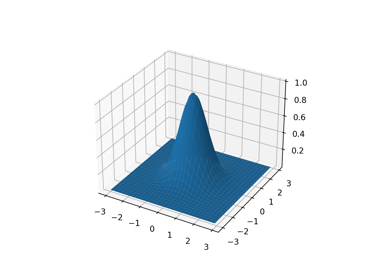
class leap_ec.real_rep.problems.GaussianProblem(width=1, height=1, maximize=True)

A multidimensional, isotropic Gaussian function, defined by

\[A\exp\left( - \sum_i^n \left(\frac{x_i}{w}\right)^2 \right)\]

Parameters

width (float) – the width parameter \(w\)
height (float) – the height parameter \(A\)

from leap_ec.real_rep.problems import GaussianProblem, plot_2d_problem
bounds = GaussianProblem.bounds  # Some typical bounds
problem = GaussianProblem(width=1, height=1)
plot_2d_problem(problem, xlim=bounds, ylim=bounds, granularity=0.1)

(Source code, png, hires.png, pdf)

bounds = (-3, 3)

evaluate(phenome)

Evaluate the given phenome.

Practitioners must over-ride this member function.

Note that by default the individual comparison operators assume a maximization problem; if this is a minimization problem, then just negate the value when returning the fitness.

Parameters: phenome – the phenome to evaluate (this will not be modified)
Returns: the fitness value

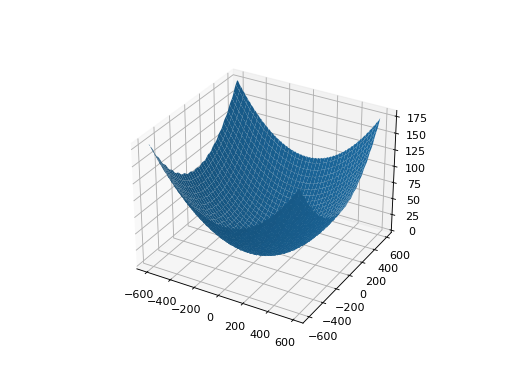
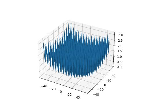
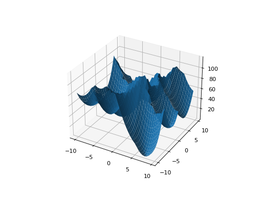
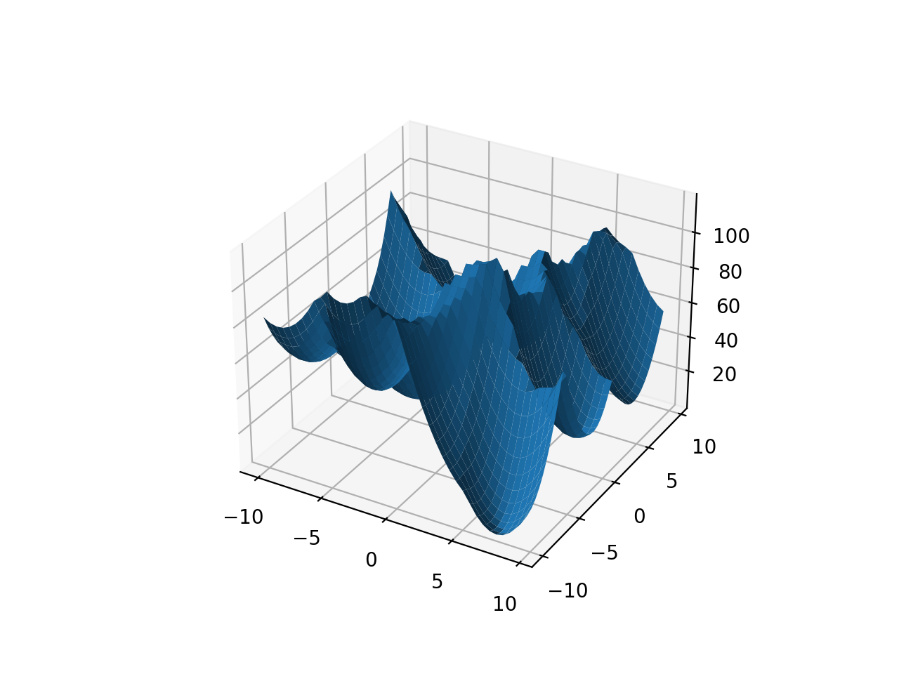
class leap_ec.real_rep.problems.GriewankProblem(maximize=False)

The classic Griewank problem. Like the RastriginProblem function, the Griewank has a quadratic global structure with many local optima that are distrib in a regular pattern.

\[f(\mathbf{x}) = \sum_{i=1}^d \frac{x_i^2}{4000} - \prod_{i=1}^d \cos\left(\frac{x_i}{\sqrt{i}}\right) + 1\]

Parameters: maximize (bool) – the function is maximized if True, else minimized.

from leap_ec.real_rep.problems import GriewankProblem, plot_2d_problem
bounds = GriewankProblem.bounds  # Contains traditional bounds
plot_2d_problem(GriewankProblem(), xlim=bounds, ylim=bounds, granularity=10)

(Source code, png, hires.png, pdf)

from leap_ec.real_rep.problems import GriewankProblem, plot_2d_problem
bounds = [-50, 50]
plot_2d_problem(GriewankProblem(), xlim=bounds, ylim=bounds, granularity=1)

(Source code, png, hires.png, pdf)

bounds = [-600, 600]

evaluate(phenome)

Computes the function value from a real-valued phenome.

Parameters: phenome – real-valued vector to be evaluated
Returns: its fitness.

class leap_ec.real_rep.problems.LangermannProblem(m=5, c=(1, 2, 5, 2, 3), a=((3, 5), (5, 2), (2, 1), (1, 4), (7, 9)), maximize=False)

A popular multi-modal test function built by summing together \(m\) terms.

\[f(\mathbf{x}) = -\sum_{i=1}^m c_i \exp\left( -\frac{1}{\pi} \sum_{j=1}^d(x_j - A_{ij})^2\right) \cos\left(\pi\sum_{j=1}^d(x_j - A_{ij})^2\right)\]

Langermann’s function is parameterized by a vector \(c_i\) of length \(m\) and a matrix \(A_{ij}\) of dimension \(m \times d\). This class uses the traditional parameterization as the default, with \(m=5\) and

\[\begin{split}c = (1, 2, 5, 2, 3) \\ A = \left[ \begin{array}{ll} 3 & 5\\ 5 & 2\\ 2 & 1\\ 1 & 4\\ 7 & 9 \end{array} \right].\end{split}\]

Parameters

m (int) – total number of terms in the function’s sum
c ([float]) – amplitude coefficients for each term
a ([[float]]) – offsets points for each term
maximize (bool) – the function is maximized if True, else minimized.

from leap_ec.real_rep.problems import LangermannProblem, plot_2d_problem
bounds = LangermannProblem.bounds  # Contains traditional bounds
plot_2d_problem(LangermannProblem(), xlim=bounds, ylim=bounds, granularity=0.2)

(Source code, png, hires.png, pdf)

bounds = [0, 10]

default_a = ((3, 5), (5, 2), (2, 1), (1, 4), (7, 9))

evaluate(phenome)

Computes the function value from a real-valued phenome.

Parameters: phenome – real-valued vector to be evaluated
Returns: its fitness.

class leap_ec.real_rep.problems.LunacekProblem(N, d=1.0, mu_1=2.5, mu_2=None, s=None, maximize=False)

Lunacek’s function is also know as the “double Rastrigin” or “bi-Rastrigin” problem, because it overlays a RastriginProblem-style cosine function across a pair of spheroid functions.

This function was designed to model the double-funnel macrostructure that occurs in some difficult cases of the Lennard-Jones function (a famous function from molecular dynamics).

\[f(\mathbf{x}) = \min \left( \left\{ \sum_{i=1}^N(x_i - \mu_1)^2 \right\}, \left\{ d \cdot N + s \cdot \sum_{i=1}^N(x_i - \mu_2)^2\right\} \right) + 10\sum_{i=1}^N(1 - \cos(2\pi(x_i-\mu_i))),\]

where \(N\) is the dimensionality of the solution vector, and the second sphere center parameter \(\mu_2\) is typically given by

\[\mu_2 = -\sqrt{\frac{\mu_1^2 - d}{s}}\]

and \(s\) is by default a function on \(N\):

\[s = 1 - \frac{1}{2\sqrt{N + 20} - 8.2}\]

These respective defaults are used for \(\mu_2\) and \(s\) whenever mu_2 and s are set to None.

Because of these complicated defaults, this class requires that you explicitly set the dimensionality of \(N\) of the expected input solutions. A warning will be thrown if an input solution is encountered that doesn’t match the expected dimensionality.

Parameters

N (int) – dimensionality of the anticipated input solutions
d (float) – base fitness value of the second spheroid
mu_1 (float) – offset of the first spheroid
mu_2 (float) – offset of the second spheroid (if None, this will be calculated automatically)
s (float) – scale parameter for the second spheroid (if None, this will be calculated automatically)
maximize (bool) – the function is maximized if True, else minimized.

from leap_ec.real_rep.problems import LunacekProblem, plot_2d_problem
bounds = LunacekProblem.bounds  # Contains traditional bounds
plot_2d_problem(LunacekProblem(N=2), xlim=bounds, ylim=bounds, granularity=0.1)

(Source code, png, hires.png, pdf)

bounds = (-5, 5)

evaluate(phenome)

Computes the function value from a real-valued phenome.

Parameters: phenome – real-valued vector to be evaluated
Returns: its fitness.

class leap_ec.real_rep.problems.MatrixTransformedProblem(problem, matrix, maximize=None)

Apply a linear transformation to a fitness function.

Parameters: matrix – an nxn matrix, where n is the genome length.
Returns: a function that first applies -matrix to the input, then applies fun to the transformed input.

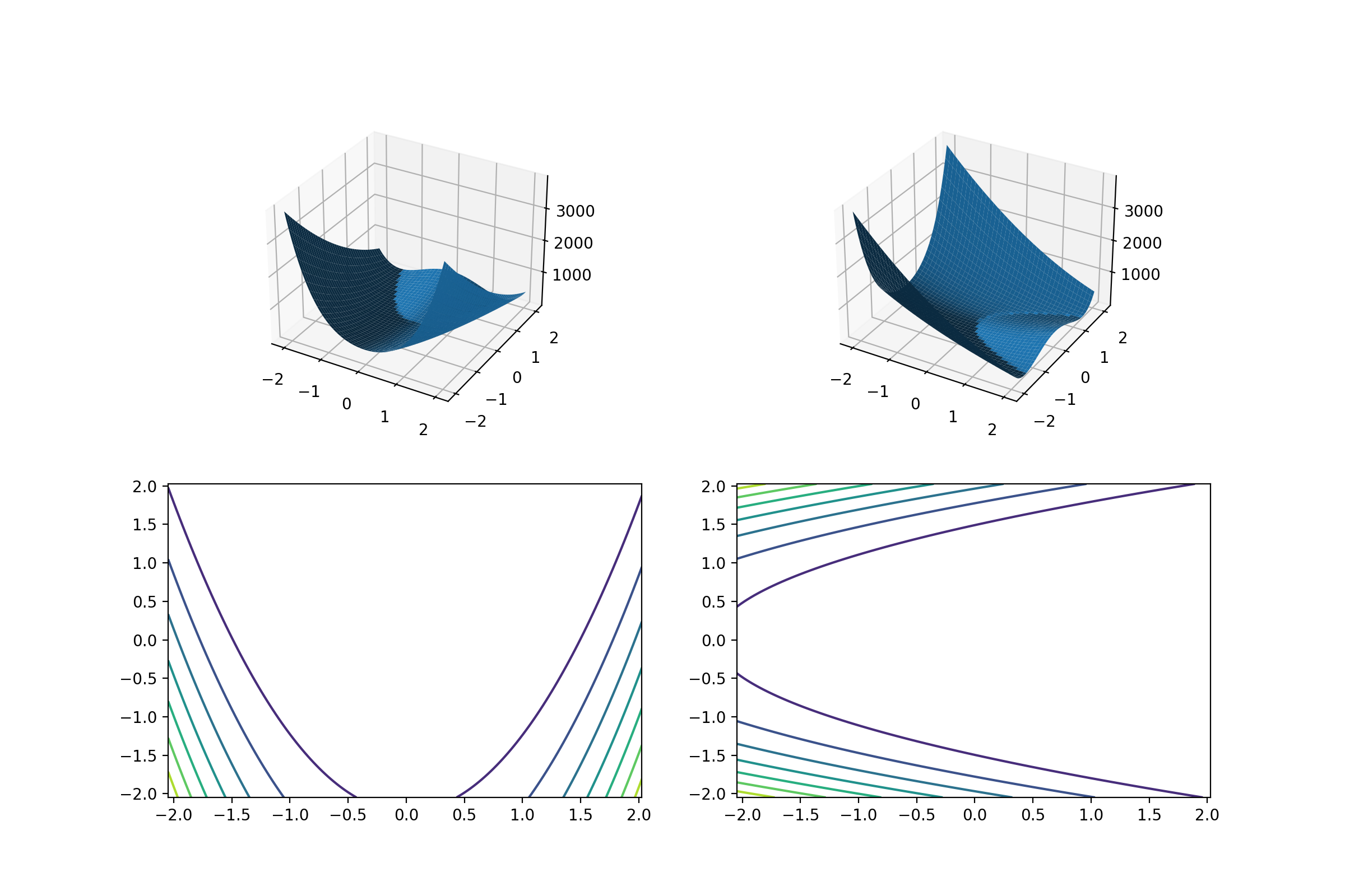
For example, here we manually construct a 2x2 rotation matrix and apply it to the leap.RosenbrockProblem function:

from matplotlib import pyplot as plt
from leap_ec.real_rep.problems import RosenbrockProblem, MatrixTransformedProblem, plot_2d_problem

original_problem = RosenbrockProblem()
theta = np.pi/2
matrix = [[np.cos(theta), -np.sin(theta)],                 [np.sin(theta), np.cos(theta)]]

transformed_problem = MatrixTransformedProblem(original_problem, matrix)

fig = plt.figure(figsize=(12, 8))

plt.subplot(221, projection='3d')
bounds = RosenbrockProblem.bounds  # Contains traditional bounds
plot_2d_problem(original_problem, xlim=bounds, ylim=bounds, ax=plt.gca(), granularity=0.025)

plt.subplot(222, projection='3d')
plot_2d_problem(transformed_problem, xlim=bounds, ylim=bounds, ax=plt.gca(), granularity=0.025)

plt.subplot(223)
plot_2d_problem(original_problem, kind='contour', xlim=bounds, ylim=bounds, ax=plt.gca(), granularity=0.025)

plt.subplot(224)
plot_2d_problem(transformed_problem, kind='contour', xlim=bounds, ylim=bounds, ax=plt.gca(), granularity=0.025)

(Source code, png, hires.png, pdf)

evaluate(phenome)

Evaluated the fitness of a point on the transformed fitness landscape.

For example, consider a sphere function whose global optimum is situated at (0, 1):

>>> import numpy as np
>>> s = TranslatedProblem(SpheroidProblem(), offset=[0, 1])
>>> round(s.evaluate(np.array([0, 1])), 5)
0

Now let’s take a rotation matrix that transforms the space by pi/2 radians:

>>> import numpy as np
>>> theta = np.pi/2
>>> matrix = [[np.cos(theta), -np.sin(theta)],                      [np.sin(theta), np.cos(theta)]]
>>> r = MatrixTransformedProblem(s, matrix)

The rotation has moved the new global optimum to (1, 0)

>>> round(r.evaluate(np.array([1, 0])), 5)
0.0

The point (0, 1) lies at a distance of sqrt(2) from the new optimum, and has a fitness of 2:

>>> round(r.evaluate(np.array([0, 1])), 5)
2.0

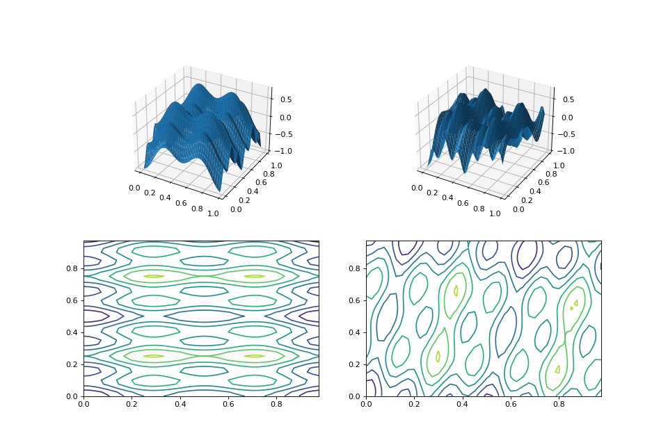
classmethod random_orthonormal(problem, dimensions, maximize=None)

Create a MatrixTransformedProblem that performs a random rotation and/or inversion of the function.

We accomplish this by generating a random orthonormal basis for R^n and plugging the resulting matrix into MatrixTransformedProblem.

The classic algorithm we use here is based on the Gramm-Schmidt process: we first generate a set of random vectors, and then convert them into an orthonormal basis. This approach is described in Hansen and Ostermeier’s original CMA-ES paper:

“Completely derandomized self-adaptation in evolution strategies.” Evolutionary Computation 9.2 (2001): 159-195.

Parameters

problem – the original ScalarProblem to apply the transform to.
dimensions (int) – the number of elements each vector should have.
maximize (bool) – whether to maximize or minimize the resulting fitness function. Defaults to whatever setting the underlying problem uses.

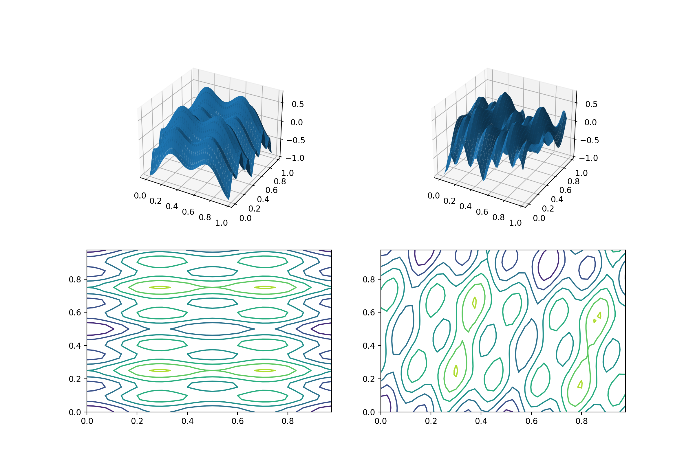
from matplotlib import pyplot as plt
from leap_ec.real_rep.problems import CosineFamilyProblem, MatrixTransformedProblem, plot_2d_problem

original_problem = CosineFamilyProblem(alpha=1.0, global_optima_counts=[2, 3], local_optima_counts=[2, 3])

transformed_problem = MatrixTransformedProblem.random_orthonormal(original_problem, 2)

fig = plt.figure(figsize=(12, 8))

plt.subplot(221, projection='3d')
bounds = original_problem.bounds
plot_2d_problem(original_problem, xlim=bounds, ylim=bounds, ax=plt.gca(), granularity=0.025)

plt.subplot(222, projection='3d')
plot_2d_problem(transformed_problem, xlim=bounds, ylim=bounds, ax=plt.gca(), granularity=0.025)

plt.subplot(223)
plot_2d_problem(original_problem, kind='contour', xlim=bounds, ylim=bounds, ax=plt.gca(), granularity=0.025)

plt.subplot(224)
plot_2d_problem(transformed_problem, kind='contour', xlim=bounds, ylim=bounds, ax=plt.gca(), granularity=0.025)

(Source code, png, hires.png, pdf)

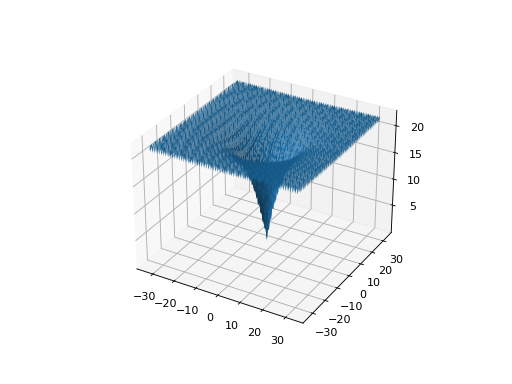
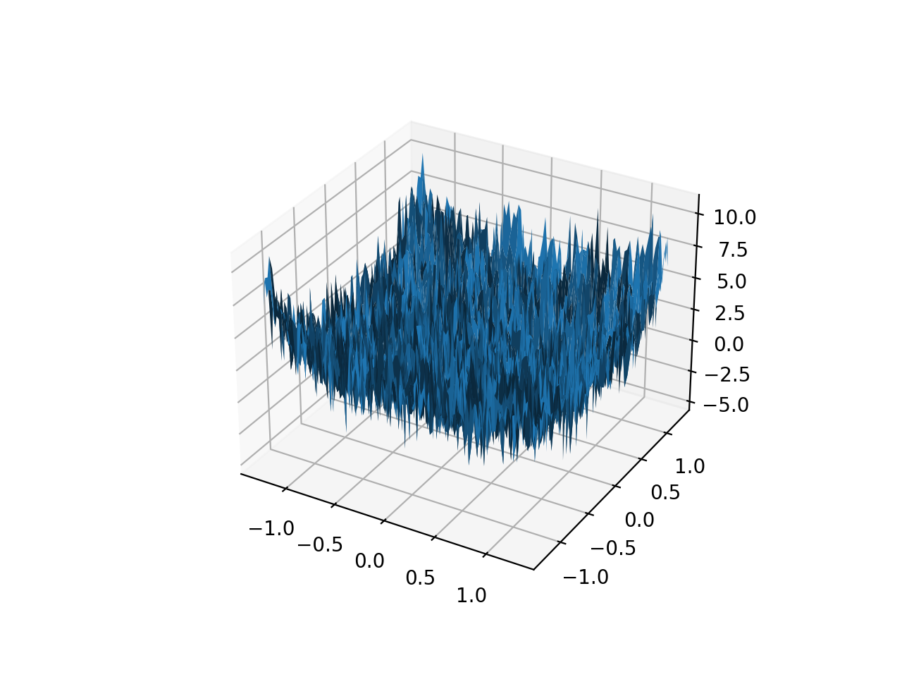
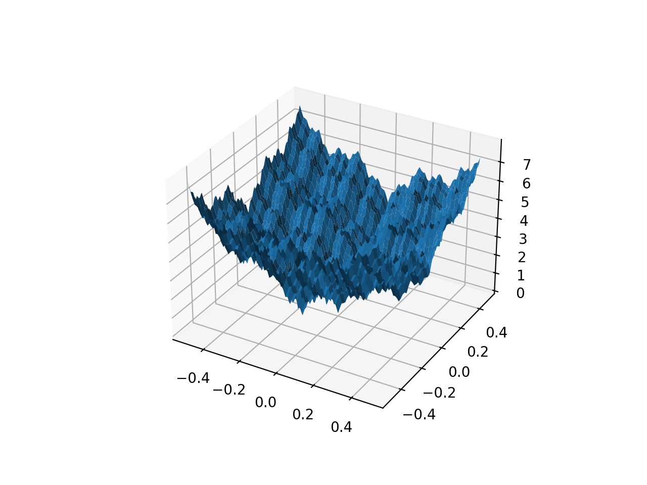
class leap_ec.real_rep.problems.NoisyQuarticProblem(maximize=False)

The classic ‘quadratic quartic’ function with Gaussian noise:

\[f(\mathbf{x}) = \sum_{i=1}^{n} i x_i^4 + \texttt{gauss}(0, 1)\]

Parameters: maximize (bool) – the function is maximized if True, else minimized.

from leap_ec.real_rep.problems import NoisyQuarticProblem, plot_2d_problem
bounds = NoisyQuarticProblem.bounds  # Contains traditional bounds
plot_2d_problem(NoisyQuarticProblem(), xlim=bounds, ylim=bounds, granularity=0.025)

(Source code, png, hires.png, pdf)

bounds = (-1.28, 1.28)

evaluate(phenome)

Computes the function value from a real-valued list phenome (the output varies, since the function has noise):

>>> phenome = [3.5, -3.8, 5.0]
>>> r = NoisyQuarticProblem().evaluate(phenome)
>>> print(f'Result: {r}')
Result: ...

Parameters: phenome – real-valued vector to be evaluated
Returns: its fitness

worse_than(first_fitness, second_fitness)

We minimize by default:

>>> s = NoisyQuarticProblem()
>>> s.worse_than(100, 10)
True

>>> s = NoisyQuarticProblem(maximize=True)
>>> s.worse_than(100, 10)
False

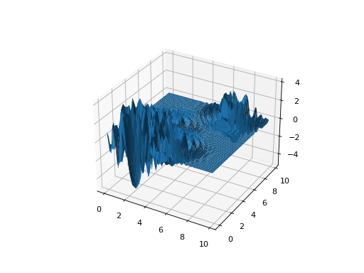
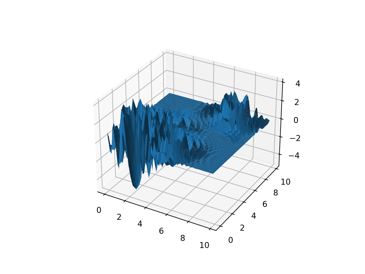
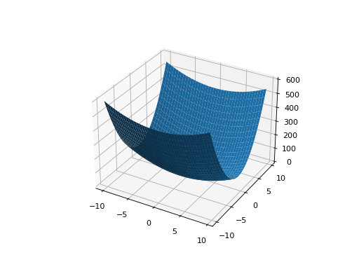
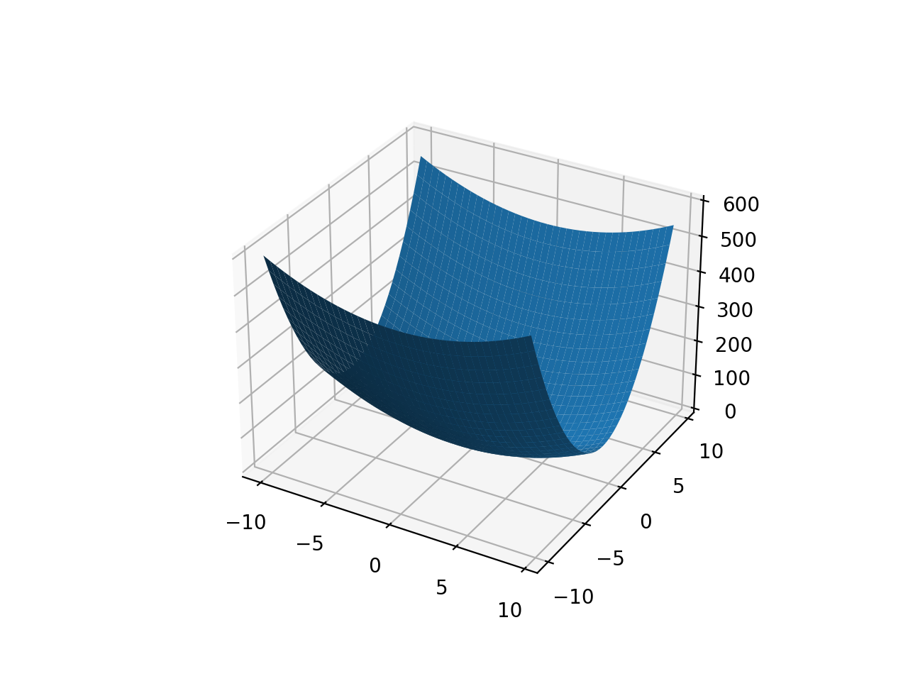
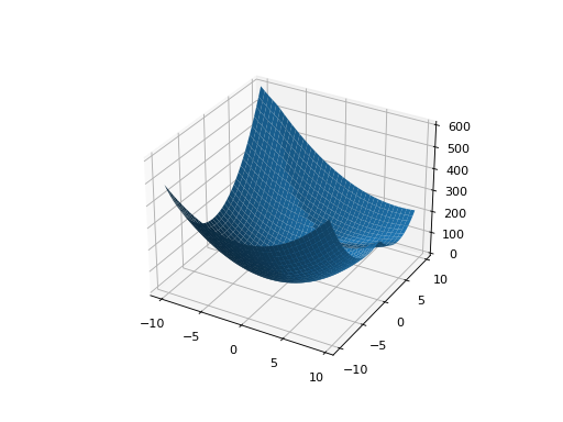
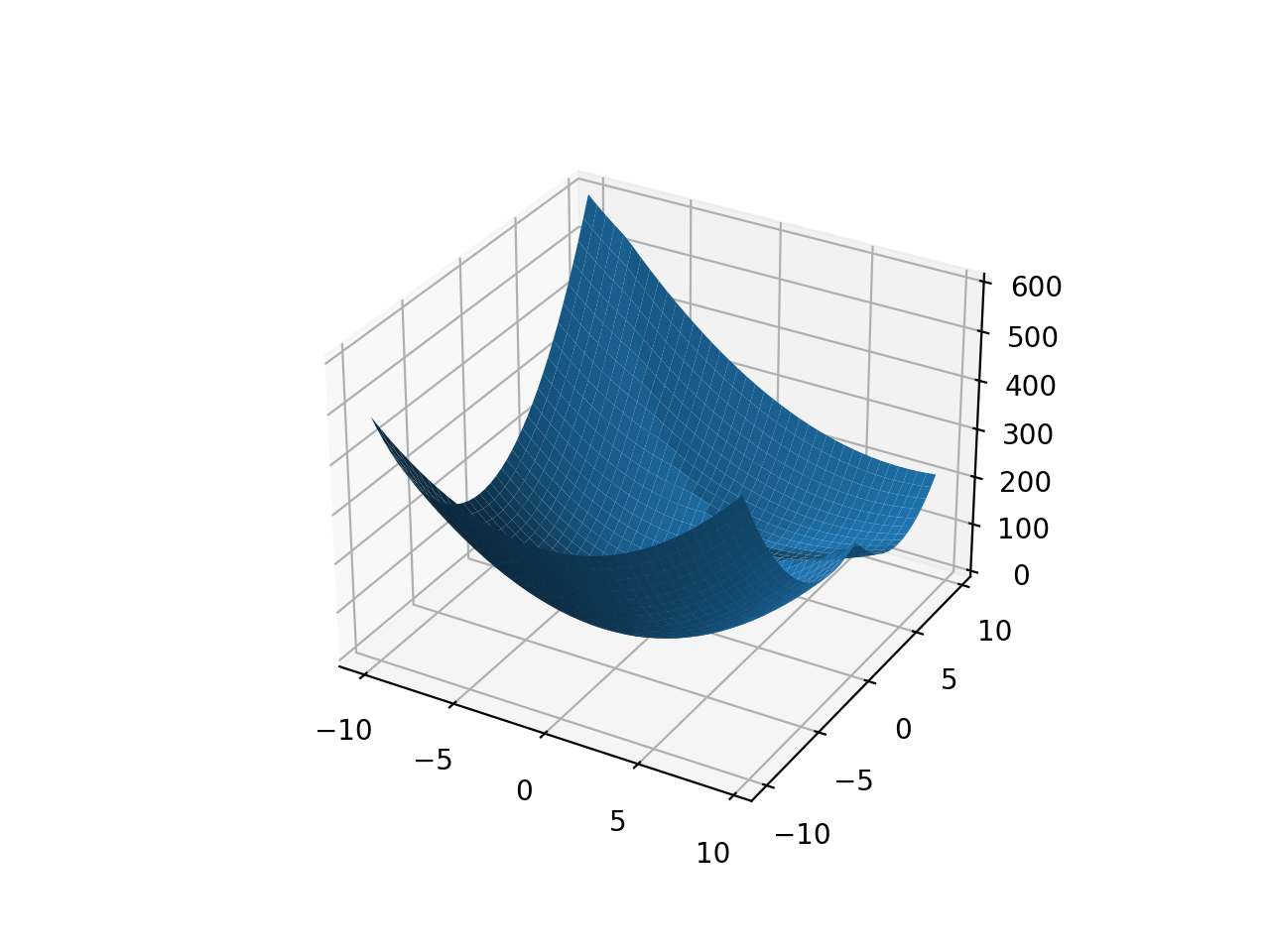
class leap_ec.real_rep.problems.ParabaloidProblem(diagonal_matrix: ndarray, rotation_matrix: ndarray, maximize=False)

A generalization of the SpheroidProblem into parabaloids (including elliptic and hyperbolic parabaloids).

We construct the parabaloid by combining a diagonal matrix (which defines an axis-aligned parabaloid) with an orthornormal rotation. Together, these make up the eigenvalues and eigenbasis, respectively, of an arbitrary parabaloid:

\[\mathbf{A} = \mathbf{R}^\top \mathbf{D} \mathbf{R}\]

We then compute fitness by interpretting \(A\) as a quadratic form:

\[f(x) = x^\top \mathbf{A} x\]

When the eigenvalues are all positive, then the result is an elliptic parabaloid

from leap_ec.real_rep .problems import ParabaloidProblem, plot_2d_problem
from matplotlib import pyplot as plt
import numpy as np

p = ParabaloidProblem(diagonal_matrix=np.diag([1, 5]), rotation_matrix=np.identity(2))
plot_2d_problem(p, xlim=(-10, 10), ylim=(-10, 10), granularity=0.5)
plt.show()

(Source code, png, hires.png, pdf)

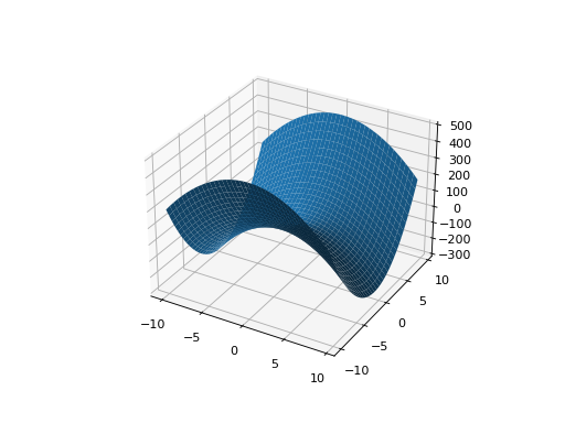
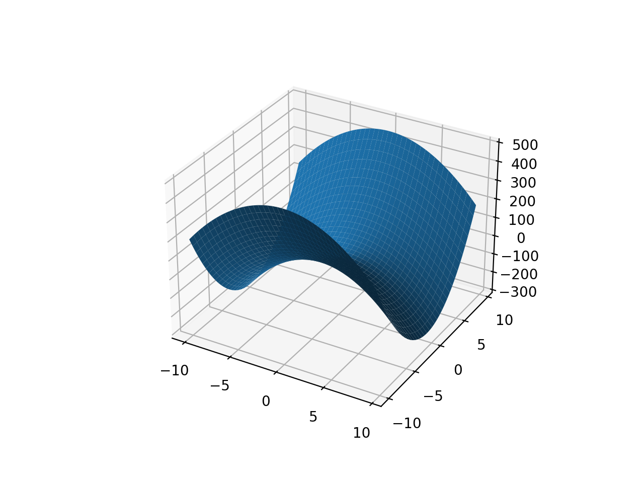
If one or more eigenvalues are negative, then a hyperbolic parabloid results, which has a saddle shape:

from leap_ec.real_rep .problems import ParabaloidProblem, plot_2d_problem
from matplotlib import pyplot as plt
import numpy as np

p = ParabaloidProblem(diagonal_matrix=np.diag([-3, 5]), rotation_matrix=np.identity(2))
plot_2d_problem(p, xlim=(-10, 10), ylim=(-10, 10), granularity=0.5)
plt.show()

(Source code, png, hires.png, pdf)

evaluate(phenome)

Evaluate the given phenome.

Practitioners must over-ride this member function.

Note that by default the individual comparison operators assume a maximization problem; if this is a minimization problem, then just negate the value when returning the fitness.

Parameters: phenome – the phenome to evaluate (this will not be modified)
Returns: the fitness value

class leap_ec.real_rep.problems.QuadraticFamilyProblem(diagonal_matrices: list, rotation_matrices: list, offset_vectors: list, fitness_offsets: list, maximize=False)

A configurable multi-modal function based on combinations of spheroids or parabaloids. Taken from the problem generators proposed by Rönkkönen et al. [RonkkonenLKL08].

The function is given by

\[f(\mathbf{x}) = \min_{i=1,2,\dots,q} \left( (\mathbf{x} - \mathbf{p}_i)^\top \mathbf{B}_i^{-1} (\mathbf{x} - \mathbf{p}_i) + v_i \right)\]

where the \(\mathbf{p}_i\) gives the center of each quadratic (i.e. the location of each local minimum), the \(v_i\) give their fitness values, and the \(\mathbf{B}_i^{-1}\) are symmetric matrices.

The easiest way to create one of these problems is to use the random generator:

from leap_ec.real_rep.problems import QuadraticFamilyProblem, plot_2d_problem
from matplotlib import pyplot as plt

problem = QuadraticFamilyProblem.generate(dimensions=2, num_basins=30)
plot_2d_problem(problem, xlim=(-10, 10), ylim=(-10, 10), granularity=0.5)
plt.show()

(Source code, png, hires.png, pdf)

You can also specify the problem structure directly by providing two matrices for each parabaloid along with an offset vector (for translation) and a scalar offset (to define the minimum fitness value for the basin):

from leap_ec.real_rep.problems import QuadraticFamilyProblem, plot_2d_problem, random_orthonormal_matrix
from matplotlib import pyplot as plt
import numpy as np

# Define the parameters for each parabaloid

diag1 = np.diag([2, 4])     # Diagonal matrix defining the widths (eigenvalues) of the basin for each dimension
rot1 = np.identity(2)       # Rotation matrix, in this case the identity (no rotation)
offset1 = np.array([-1, -1])  # Offset used to translate the basin location
fitness1 = 0                # Fitness value of the local optimum

diag2 = np.diag([5, 1])
rot2 = random_orthonormal_matrix(dimensions=2)  # Apply a random rotation to the second basin
offset2 = np.array([3, 4])
fitness2 = 100.0

# Build the problem
problem = QuadraticFamilyProblem(
    diagonal_matrices = [ diag1, diag2 ],
    rotation_matrices = [ rot1, rot2 ],
    offset_vectors = [ offset1, offset2 ],
    fitness_offsets = [ fitness1, fitness2 ]
)

# Visualize
plot_2d_problem(problem, xlim=(-10, 10), ylim=(-10, 10), granularity=0.5)
plt.show()

(Source code, png, hires.png, pdf)

property dimensions

evaluate(phenome)

Evaluate the given phenome.

Practitioners must over-ride this member function.

Note that by default the individual comparison operators assume a maximization problem; if this is a minimization problem, then just negate the value when returning the fitness.

Parameters: phenome – the phenome to evaluate (this will not be modified)
Returns: the fitness value

classmethod generate(dimensions: int, num_basins: int, num_global_optima: int = 1, width_bounds: tuple = (1, 5), offset_bounds: tuple = (-10, 10), fitness_offset_bounds: tuple = (10, 100))

Convenient method to generate a QuadraticFamilyProblem by randomly sampling the matrices that define it.

>>> problem = QuadraticFamilyProblem.generate(10, 20, num_global_optima = 2)
>>> x = problem.evaluate(np.array([0.0, 0.5, 0.0, 0.6, 0.0, 0.7, 0.6, 0.8, 4.3, 0.2]))

property num_basins

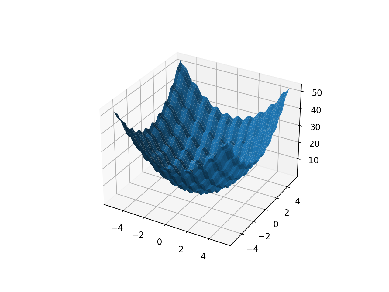
class leap_ec.real_rep.problems.RastriginProblem(a=1.0, maximize=False)

The classic Rastrigin problem. The Rastrigin provides a real-valued fitness landscape with a quadratic global structure (like the SpheroidProblem), plus a sinusoidal local structure with many local optima.

\[f(\vec{x}) = An + \sum_{i=1}^n x_i^2 - A\cos(2\pi x_i)\]

Parameters: maximize (bool) – the function is maximized if True, else minimized.

from leap_ec.real_rep.problems import RastriginProblem, plot_2d_problem
bounds = RastriginProblem.bounds  # Contains traditional bounds
plot_2d_problem(RastriginProblem(), xlim=bounds, ylim=bounds, granularity=0.025)

(Source code, png, hires.png, pdf)

bounds = (-5.12, 5.12)

evaluate(phenome)

Computes the function value from a real-valued list phenome:

>>> phenome = [1.0/12, 0]
>>> RastriginProblem().evaluate(phenome) 
0.1409190406...

Parameters: phenome – real-valued vector to be evaluated
Returns: its fitness

worse_than(first_fitness, second_fitness)

We minimize by default:

>>> s = RastriginProblem()
>>> s.worse_than(100, 10)
True

>>> s = RastriginProblem(maximize=True)
>>> s.worse_than(100, 10)
False

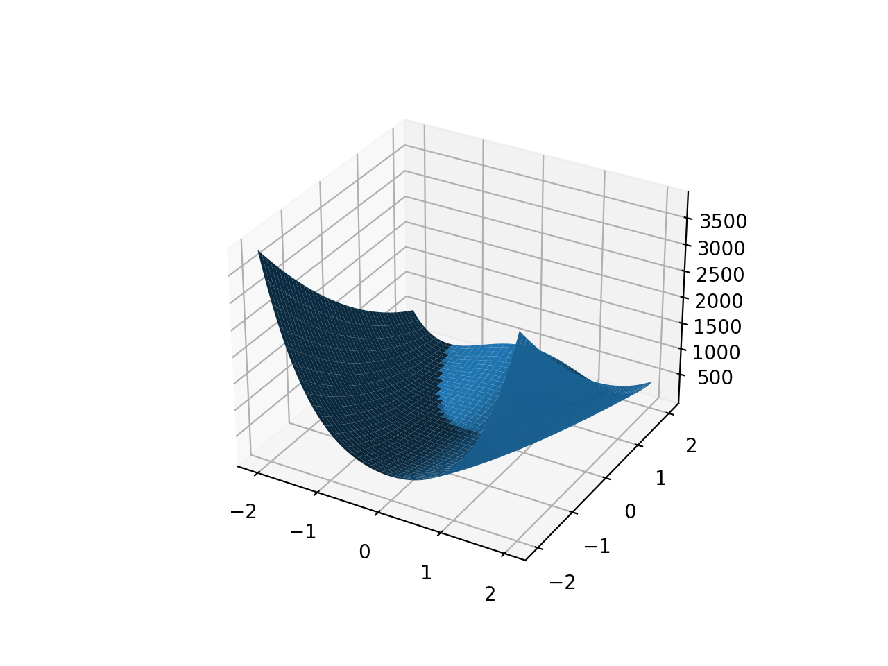
class leap_ec.real_rep.problems.RosenbrockProblem(maximize=False)

The classic RosenbrockProblem problem, a.k.a. the “banana” or “valley” function.

\[f(\mathbf{x}) = \sum_{i=1}^{d-1} \left[ 100 (x_{i + 1} - x_i^2)^2 + (x_i - 1)^2\right]\]

Parameters: maximize (bool) – the function is maximized if True, else minimized.

from leap_ec.real_rep.problems import RosenbrockProblem, plot_2d_problem
bounds = RosenbrockProblem.bounds  # Contains traditional bounds
plot_2d_problem(RosenbrockProblem(), xlim=bounds, ylim=bounds, granularity=0.025)

(Source code, png, hires.png, pdf)

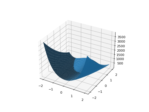
bounds = (-2.048, 2.048)

evaluate(phenome)

Computes the function value from a real-valued list phenome:

>>> phenome = [0.5, -0.2, 0.1]
>>> RosenbrockProblem().evaluate(phenome)
22.3

Parameters: phenome – real-valued vector to be evaluated
Returns: its fitness

worse_than(first_fitness, second_fitness)

We minimize by default:

>>> s = RosenbrockProblem()
>>> s.worse_than(100, 10)
True

>>> s = RosenbrockProblem(maximize=True)
>>> s.worse_than(100, 10)
False

class leap_ec.real_rep.problems.ScaledProblem(problem, new_bounds, maximize=None)

Scale the search space of a fitness function up or down.

evaluate(phenome)

Evaluate the given phenome.

Practitioners must over-ride this member function.

Note that by default the individual comparison operators assume a maximization problem; if this is a minimization problem, then just negate the value when returning the fitness.

Parameters: phenome – the phenome to evaluate (this will not be modified)
Returns: the fitness value

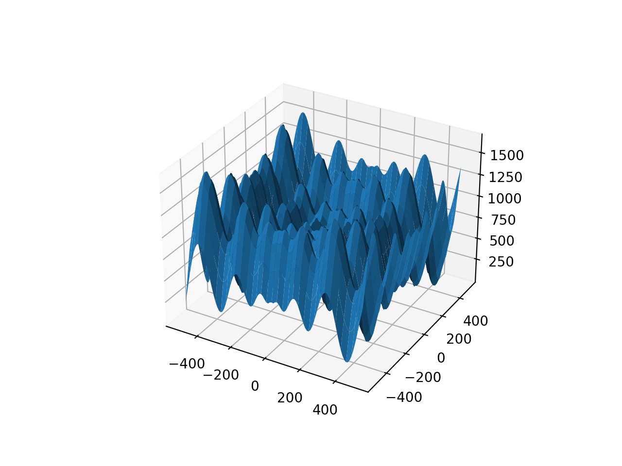
class leap_ec.real_rep.problems.SchwefelProblem(alpha=418.982887, maximize=False)

Schwefel’s function is another traditional multimodal test function whose local optima are distributed in a slightly irregular way, and whose global optimum is out at the edge of the search space (with no gently sloping macrostructure to guide the algorithm toward it).

Compare this to the RastriginProblem function, whose global optimum lies at the center of a quadratic bowl with a regular grid of local optima.

\[f(\mathbf{x}) = \sum_{i=1}^d\left(-x_i \cdot\sin\left(\sqrt{|x_i|} \right)\right) + \alpha \cdot d\]

Parameters

alpha (float) – fitness offset (the default value ensures that the global optimum has zero fitness)
maximize (bool) – the function is maximized if True, else minimized.

from leap_ec.real_rep.problems import SchwefelProblem, plot_2d_problem
bounds = SchwefelProblem.bounds  # Contains traditional bounds
plot_2d_problem(SchwefelProblem(), xlim=bounds, ylim=bounds, granularity=10)

(Source code, png, hires.png, pdf)

bounds = (-512, 512)

evaluate(phenome)

Computes the function value from a real-valued phenome.

Parameters: phenome – phenome with a real-valued phenome to be evaluated
Returns: its fitness.

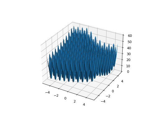
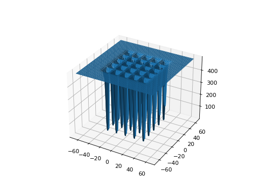
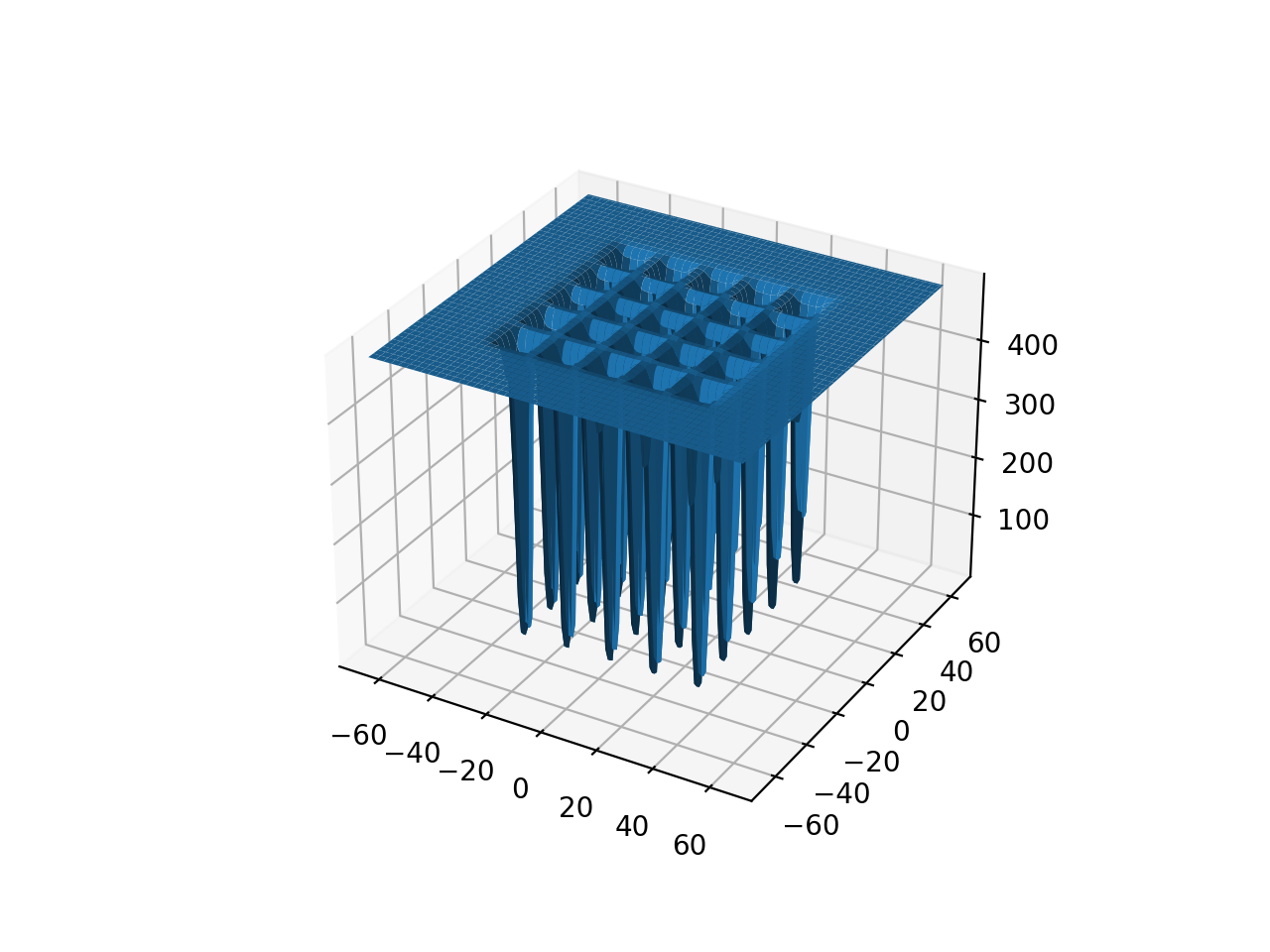
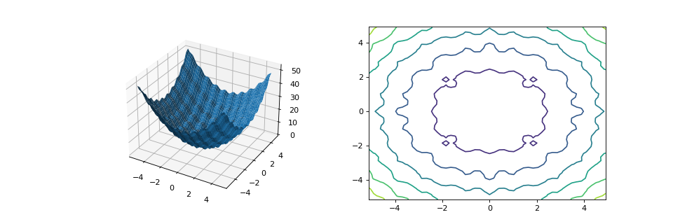
class leap_ec.real_rep.problems.ShekelProblem(k=500, c=array([1, 2, 3, 4, 5, 6, 7, 8, 9, 10, 11, 12, 13, 14, 15, 16, 17, 18, 19, 20, 21, 22, 23, 24, 25]), maximize=False)

The classic ‘Shekel’s foxholes’ function.

\[f(\mathbf{x}) = \frac{1}{\frac{1}{K} + \sum_{j=1}^{25} \frac{1}{f_j(\mathbf{x})}}\]

where

\[f_j(\mathbf{x}) = c_j + \sum_{i=1}^2 (x_i - a_{ij})^6\]

and the points \(\left\{ (a_{1j}, a_{2j})\right\}_{j=1}^{25}\) define the functions various optima, and are given by the following hardcoded matrix:

\[\begin{split}\left[a_{ij}\right] = \left[ \begin{array}{lllllllllll} -32 & -16 & 0 & 16 & 32 & -32 & -16 & \cdots & 0 & 16 & 32 \\ -32 & -32 & -32 & -32 & -32 & -16 & -16 & \cdots & 32 & 32 & 32 \end{array} \right].\end{split}\]

Parameters

k (int) – the value of \(K\) in the fitness function.
c ([int]) – list of values for the function’s \(c_j\) parameters. Each c[j] approximately corresponds to the depth of the jth foxhole.
maximize (bool) – the function is maximized if True, else minimized.
maximize – the function is maximized if True, else minimized.

from leap_ec.real_rep.problems import ShekelProblem, plot_2d_problem
bounds = ShekelProblem.bounds  # Contains traditional bounds
plot_2d_problem(ShekelProblem(), xlim=bounds, ylim=bounds, granularity=0.9)

(Source code, png, hires.png, pdf)

bounds = (-65.536, 65.536)

evaluate(phenome)

Computes the function value from a real-valued list phenome (the output varies, since the function has noise).

Parameters: phenome – real-valued to be evaluated
Returns: its fitness

points = array([[-32, -16, 0, 16, 32, -32, -16, 0, 16, 32, -32, -16, 0, 16, 32, -32, -16, 0, 16, 32, -32, -16, 0, 16, 32], [-32, -32, -32, -32, -32, -16, -16, -16, -16, -16, 0, 0, 0, 0, 0, 16, 16, 16, 16, 16, 32, 32, 32, 32, 32]])

worse_than(first_fitness, second_fitness)

We minimize by default:

>>> s = ShekelProblem()
>>> s.worse_than(100, 10)
True

>>> s = ShekelProblem(maximize=True)
>>> s.worse_than(100, 10)
False

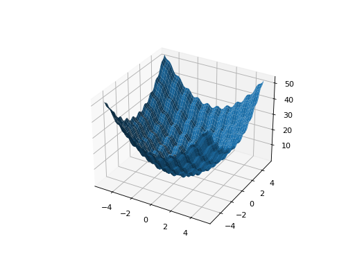
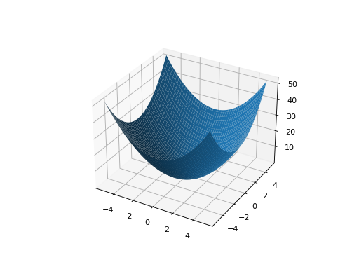
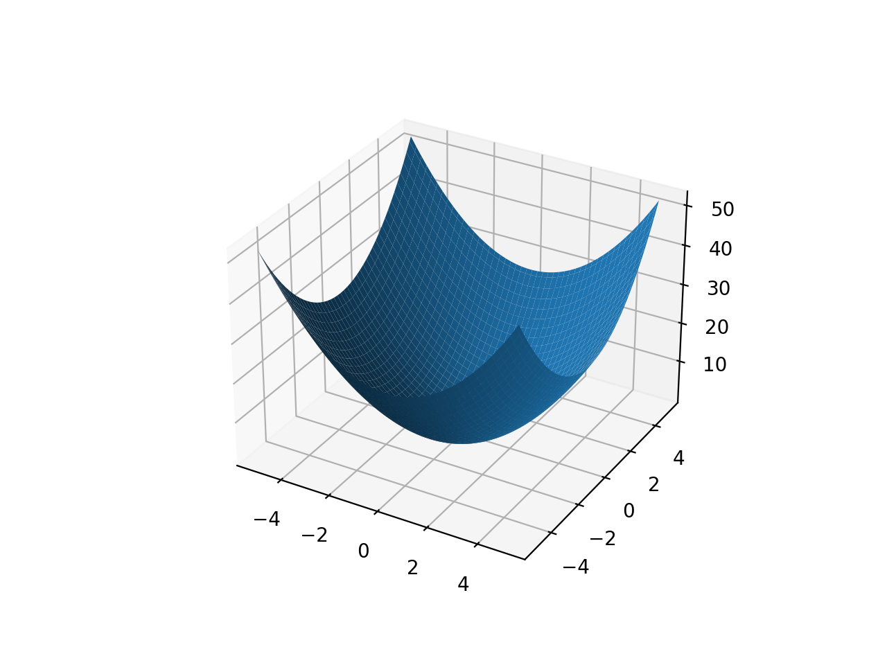
class leap_ec.real_rep.problems.SpheroidProblem(maximize=False)

Classic paraboloid function, known as the “sphere” or “spheroid” problem, because its equal-fitness contours form (hyper)spheres in n > 2.

\[f(\vec{x}) = \sum_{i}^n x_i^2\]

Parameters: maximize (bool) – the function is maximized if True, else minimized.

from leap_ec.real_rep.problems import SpheroidProblem, plot_2d_problem
bounds = SpheroidProblem.bounds  # Contains traditional bounds
plot_2d_problem(SpheroidProblem(), xlim=bounds, ylim=bounds, granularity=0.025)

(Source code, png, hires.png, pdf)

bounds = (-5.12, 5.12)

evaluate(phenome)

Computes the function value from a real-valued list phenome:

>>> phenome = [0.5, 0.8, 1.5]
>>> SpheroidProblem().evaluate(phenome)
3.14

Parameters: phenome – real-valued vector to be evaluated
Returns: it’s fitness, sum(phenome**2)

worse_than(first_fitness, second_fitness)

We minimize by default:

>>> s = SpheroidProblem()
>>> s.worse_than(100, 10)
True

>>> s = SpheroidProblem(maximize=True)
>>> s.worse_than(100, 10)
False

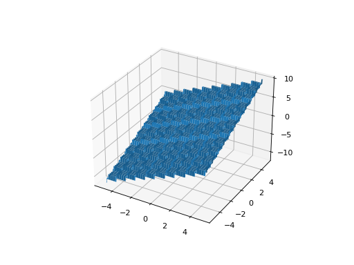
class leap_ec.real_rep.problems.StepProblem(maximize=True)

The classic ‘step’ function—a function with a linear global structure, but with stair-like plateaus at the local level.

\[f(\mathbf{x}) = \sum_{i=1}^{n} \lfloor x_i \rfloor\]

where \(\lfloor x \rfloor\) denotes the floor function.

Parameters: maximize (bool) – the function is maximized if True, else minimized.

from leap_ec.real_rep.problems import StepProblem, plot_2d_problem
bounds = StepProblem.bounds  # Contains traditional bounds
plot_2d_problem(StepProblem(), xlim=bounds, ylim=bounds, granularity=0.025)

(Source code, png, hires.png, pdf)

bounds = (-5.12, 5.12)

evaluate(phenome)

Computes the function value from a real-valued list phenome:

>>> import numpy as np
>>> phenome = np.array([3.5, -3.8, 5.0])
>>> StepProblem().evaluate(phenome)
4.0

Parameters: phenome – real-valued vector to be evaluated
Returns: its fitness

worse_than(first_fitness, second_fitness)

We maximize by default:

>>> s = StepProblem()
>>> s.worse_than(100, 10)
False

>>> s = StepProblem(maximize=False)
>>> s.worse_than(100, 10)
True

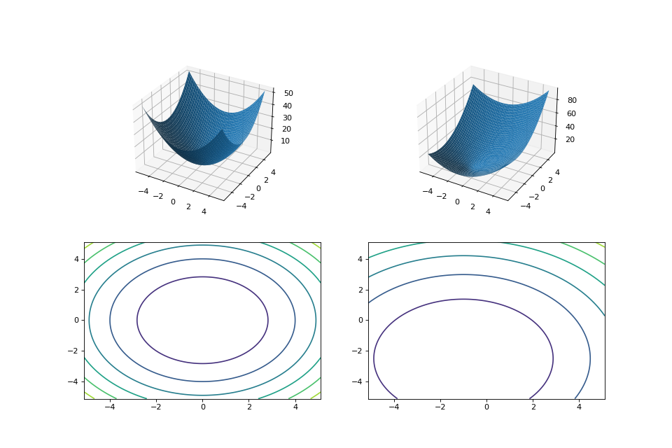
class leap_ec.real_rep.problems.TranslatedProblem(problem, offset, maximize=None)

Takes an existing fitness function and translates it by applying a fixed offset vector.

For example,

from matplotlib import pyplot as plt
from leap_ec.real_rep.problems import SpheroidProblem, TranslatedProblem, plot_2d_problem

original_problem = SpheroidProblem()
offset = [-1.0, -2.5]
translated_problem = TranslatedProblem(original_problem, offset)

fig = plt.figure(figsize=(12, 8))

plt.subplot(221, projection='3d')
bounds = SpheroidProblem.bounds  # Contains traditional bounds
plot_2d_problem(original_problem, xlim=bounds, ylim=bounds, ax=plt.gca(), granularity=0.025)

plt.subplot(222, projection='3d')
plot_2d_problem(translated_problem, xlim=bounds, ylim=bounds, ax=plt.gca(), granularity=0.025)

plt.subplot(223)
plot_2d_problem(original_problem, kind='contour', xlim=bounds, ylim=bounds, ax=plt.gca(), granularity=0.025)

plt.subplot(224)
plot_2d_problem(translated_problem, kind='contour', xlim=bounds, ylim=bounds, ax=plt.gca(), granularity=0.025)

(Source code, png, hires.png, pdf)

evaluate(phenome)

Evaluate the fitness of a point after translating the fitness function.

Translation can be used in higher than two dimensions:

>>> import numpy as np
>>> offset = [-1.0, -1.0, 1.0, 1.0, -5.0]
>>> t_sphere = TranslatedProblem(SpheroidProblem(), offset)
>>> genome = np.array([0.5, 2.0, 3.0, 8.5, -0.6])
>>> t_sphere.evaluate(genome)
90.86

classmethod random(problem, offset_bounds, dimensions, maximize=None)

Apply a random real-valued translation to a fitness function, sampled uniformly between min_offset and max_offset in every dimension.

>>> from leap_ec.real_rep.problems import TranslatedProblem, RastriginProblem, plot_2d_problem

>>> original_problem = RastriginProblem()
>>> bounds = RastriginProblem.bounds  # Contains traditional bounds
>>> translated_problem = TranslatedProblem.random(original_problem, bounds, 2)

>>> plot_2d_problem(translated_problem, kind='contour', xlim=bounds, ylim=bounds)
<matplotlib.contour...>

from leap_ec.real_rep.problems import TranslatedProblem, RastriginProblem, plot_2d_problem

original_problem = RastriginProblem()
bounds = RastriginProblem.bounds  # Contains traditional bounds
translated_problem = TranslatedProblem.random(original_problem, bounds, 2)

plot_2d_problem(translated_problem, kind='contour', xlim=bounds, ylim=bounds)

(Source code, png, hires.png, pdf)

class leap_ec.real_rep.problems.WeierstrassProblem(kmax=20, a=0.5, b=3, maximize=False)

The Weierstrass function is famous for being the first discovered example of a function that is continuous, but not differentiable. Built by adding the terms of a Fourier series, it has a jagged, self-similar structure:

\[f(\mathbf{x}) = \sum_{i=1}^d \left[ \sum_{k=0}^{kmax} a^k \cos\left( 2\pi b^k(x_i + 0.5)\right) - n \sum_{k=0}^{kmax} a^k \cos(\pi b^k) \right]\]

When used in optimization benchmarks, it’s typical to carry out the Fourier sum to kmax=20 terms.

Parameters

kmax (int) – number of terms to carry the Fourier sum out to
a (float) – amplitude parameter of the cosine terms
b (float) – wavenumber (frequency) parameter of the cosine terms
maximize (bool) – the function is maximized if True, else minimized.

from leap_ec.real_rep.problems import WeierstrassProblem, plot_2d_problem
bounds = WeierstrassProblem.bounds  # Contains traditional bounds
plot_2d_problem(WeierstrassProblem(), xlim=bounds, ylim=bounds, granularity=0.01)

(Source code, png, hires.png, pdf)

bounds = [-0.5, 0.5]

evaluate(phenome)

Computes the function value from a real-valued phenome.

Parameters: phenome – real-valued vector to be evaluated
Returns: its fitness.

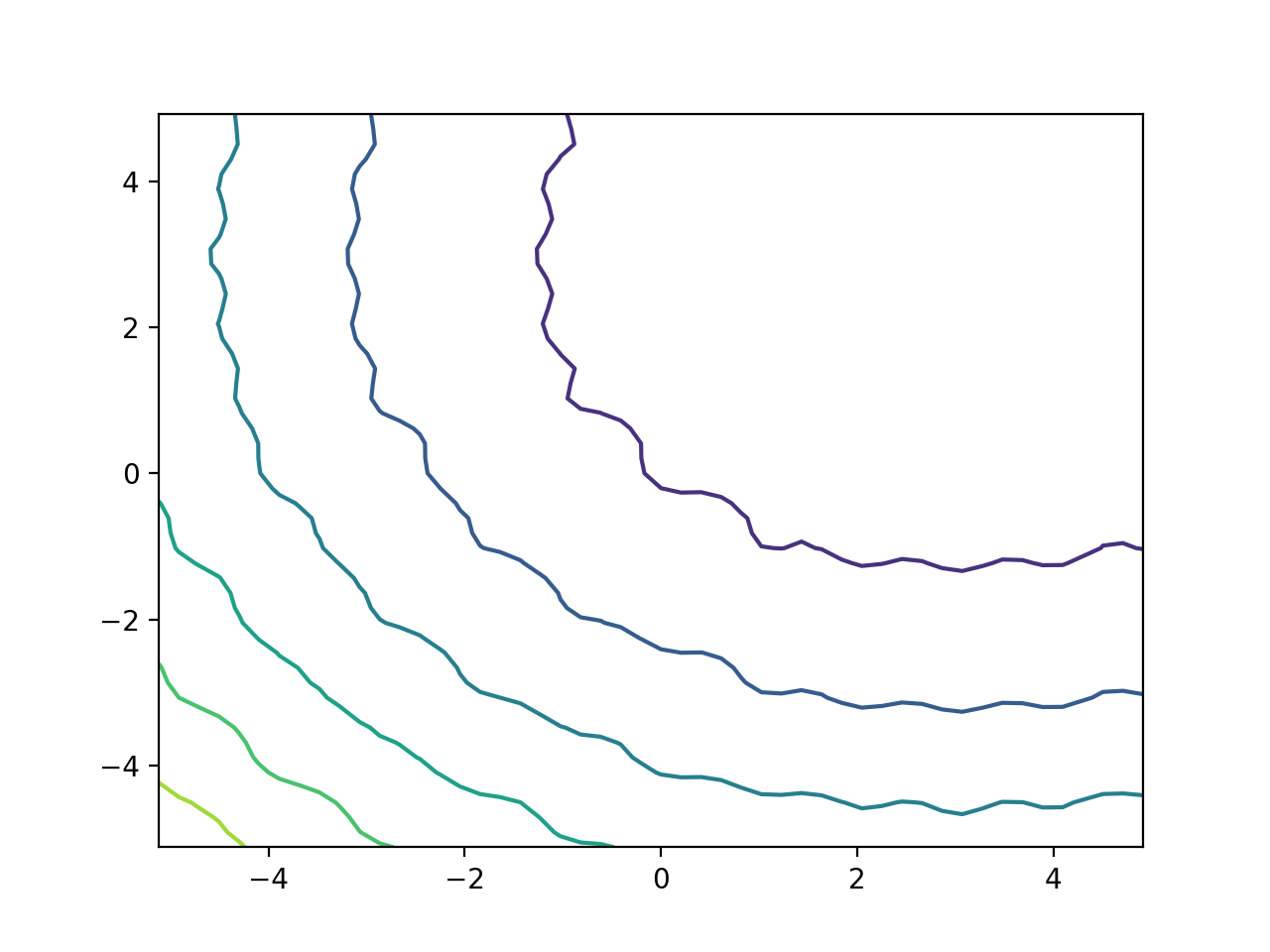
leap_ec.real_rep.problems.plot_2d_contour(fun, xlim, ylim, granularity, ax=None, title=None, pad=None)

Convenience method for plotting contours for a function that accepts 2-D real-valued inputs and produces a 1-D scalar output.

Parameters

fun (function) – The function to plot.
xlim ((float, float)) – Bounds of the horizontal axes.
ylim ((float, float)) – Bounds of the vertical axis.
ax (Axes) – Matplotlib axes to plot to (if None, a new figure will be created).
granularity (float) – Spacing of the grid to sample points along.
pad – An array of extra gene values, used to fill in the hidden dimensions with contants while drawing fitness contours.

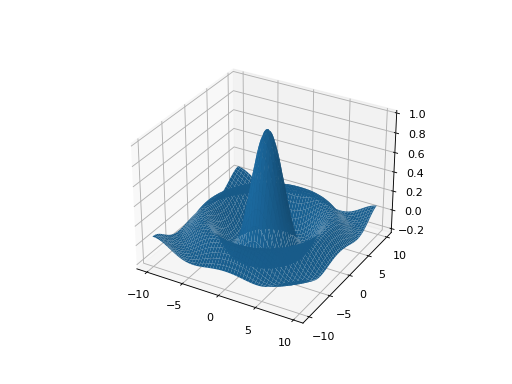
The difference between this and plot_2d_problem() is that this takes a raw function (instead of a Problem object).

import numpy as np
from scipy import linalg

from leap_ec.real_rep.problems import plot_2d_contour

def sinc_hd(phenome):
    r = linalg.norm(phenome)
    return np.sin(r)/r

plot_2d_contour(sinc_hd, xlim=(-10, 10), ylim=(-10, 10), granularity=0.2)

(Source code)

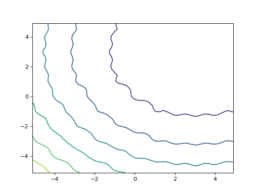
leap_ec.real_rep.problems.plot_2d_function(fun, xlim, ylim, granularity=0.1, ax=None, title=None, pad=None, **kwargs)

Convenience method for plotting a function that accepts 2-D real-valued imputs and produces a 1-D scalar output.

Parameters

fun (function) – The function to plot.
xlim ((float, float)) – Bounds of the horizontal axes.
ylim ((float, float)) – Bounds of the vertical axis.
ax (Axes) – Matplotlib axes to plot to (if None, a new figure will be created).
granularity (float) – Spacing of the grid to sample points along.
pad – An array of extra gene values, used to fill in the hidden dimensions with contants while drawing fitness contours.
kwargs – additional keyword arguments to pass along to plot_surface() or contour()

The difference between this and plot_2d_problem() is that this takes a raw function (instead of a Problem object).

import numpy as np
from scipy import linalg

from leap_ec.real_rep.problems import plot_2d_function

def sinc_hd(phenome):
    r = linalg.norm(phenome)
    return np.sin(r)/r

plot_2d_function(sinc_hd, xlim=(-10, 10), ylim=(-10, 10), granularity=0.2)

(Source code)

leap_ec.real_rep.problems.plot_2d_problem(problem, xlim=None, ylim=None, kind='surface', ax=None, granularity=None, title=None, pad=None, **kwargs)

Convenience function for plotting a Problem that accepts 2-D real-valued phenomes and produces a 1-D scalar fitness output.

Parameters

fun (Problem) – The Problem to plot.
xlim ((float, float)) – Bounds of the horizontal axes. If None, uses problem.bounds.
ylim ((float, float)) – Bounds of the vertical axis. If None, uses problem.bounds.
kind (str) – The kind of plot to create: ‘surface’ or ‘contour’
pad – An array of extra gene values, used to fill in the hidden dimensions with contants while drawing fitness contours.
ax (Axes) – Matplotlib axes to plot to (if None, a new figure will be created).
granularity (float) – Spacing of the grid to sample points along. If none is given, then the granularity will default to 1/50th of the range of the function’s bounds attribute.
kwargs – additional keyword arguments to pass along to plot_surface()

The difference between this and plot_2d_function() is that this takes a Problem object (instead of a raw function).

If no axes are specified, a new figure is created for the plot:

from leap_ec.real_rep.problems import CosineFamilyProblem, plot_2d_problem
problem = CosineFamilyProblem(alpha=1.0, global_optima_counts=[2, 2], local_optima_counts=[2, 2])
plot_2d_problem(problem, xlim=(0, 1), ylim=(0, 1), granularity=0.025);

(Source code, png, hires.png, pdf)

You can also specify axes explicitly (ex. by using ax=plt.gca(). When plotting surfaces, you must configure your axes to use projection=’3d’. Contour plots don’t need 3D axes:

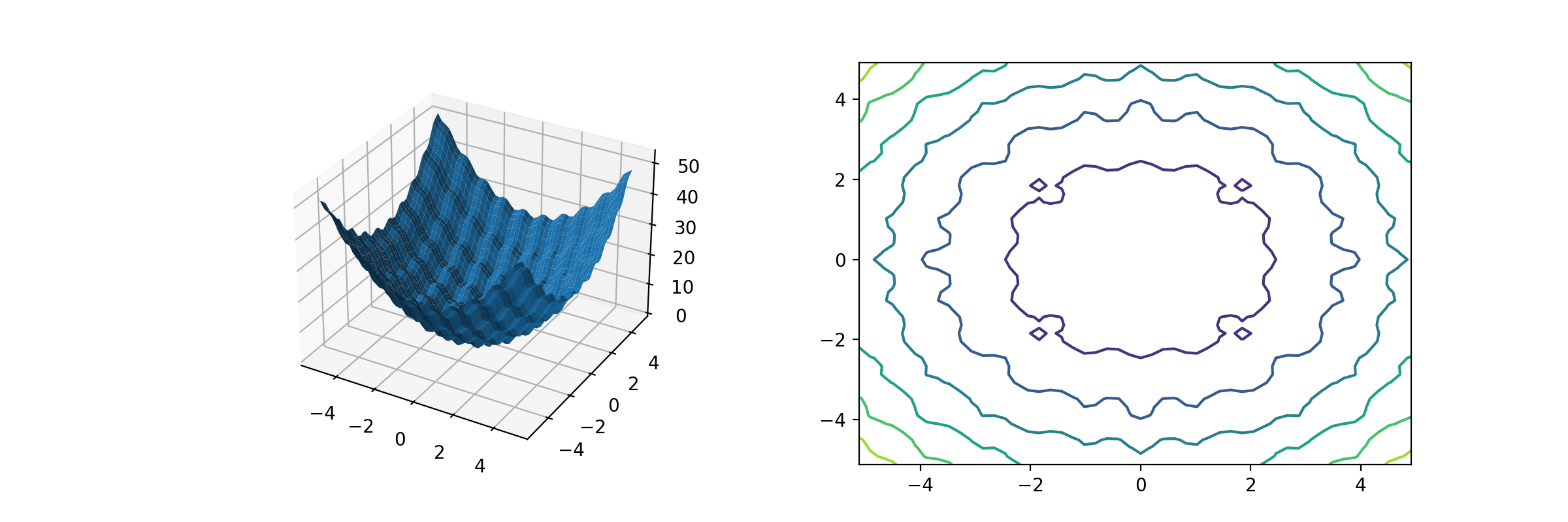
from matplotlib import pyplot as plt
from leap_ec.real_rep.problems import RastriginProblem, plot_2d_problem

fig = plt.figure(figsize=(12, 4))
bounds=RastriginProblem.bounds  # Contains default bounds

plt.subplot(121, projection='3d')
plot_2d_problem(RastriginProblem(), ax=plt.gca(), xlim=bounds, ylim=bounds)

plt.subplot(122)
plot_2d_problem(RastriginProblem(), ax=plt.gca(), kind='contour', xlim=bounds, ylim=bounds)

(Source code, png, hires.png, pdf)

leap_ec.real_rep.problems.random(size=None): Return random floats in the half-open interval [0.0, 1.0). Alias for random_sample to ease forward-porting to the new random API.

leap_ec.real_rep.problems.random_orthonormal_matrix(dimensions: int)

Generate a random orthornomal matrix using the Gramm-Schmidt process.

Orthonormal matrices represent rotations (and flips) of a space.

The defining property of an orthonormal matrix is that its transpose is its inverse:

>>> Q = random_orthonormal_matrix(10)
>>> np.allclose( Q.dot(Q.T), np.identity(10) )
True